
How to Use the ML for Trading Tools: A Labs Walkthrough
How-to article on the Feature Engineering Explorer, SHAP Explorer, and Tree Builder

The Math & Markets Labs launched last this week with three interactive ML for trading tools. Some of you asked for a walkthrough of what each tool does and how to get the most out of it. Here it is.
Tool 1: Feature Engineering Explorer
ml-feature-explorer.mathandmarkets.com
This is the companion to Post 95. It lets you do what I did in that post — test 20 candidate features and figure out which ones are signal and which ones are noise — but interactively.
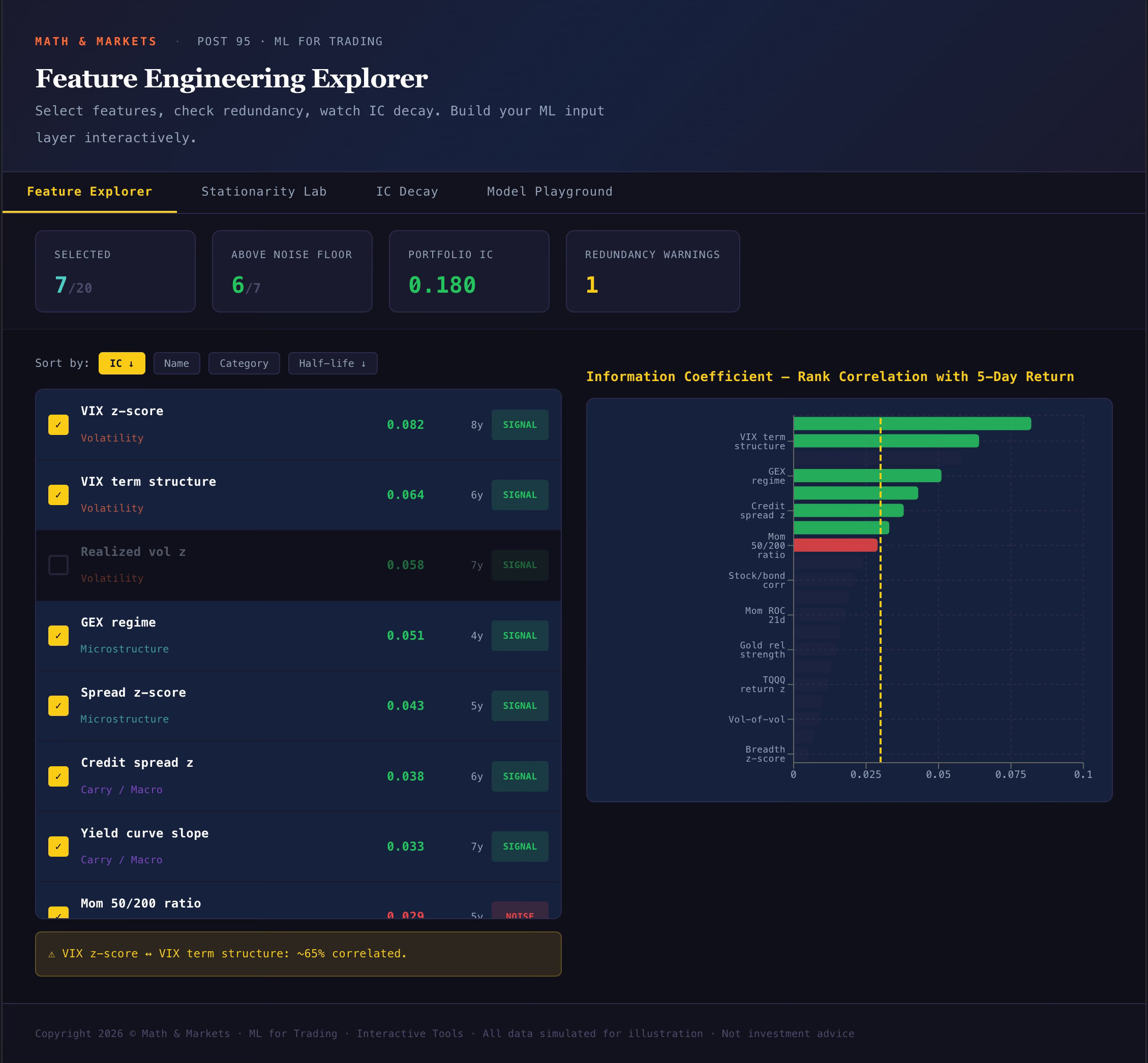
The Feature Explorer tab shows all 20 features ranked by Information Coefficient. Click any feature to select or deselect it. The scoreboard at the top updates in real-time: how many features you’ve selected, how many are above the noise floor (IC > 0.03), your portfolio’s combined IC, and how many redundancy warnings you’ve triggered. Hover over any feature to see what it measures and why it matters.
The thing to watch: redundancy warnings. If you select VIX z-score, Realized vol z, AND VIX term structure, you’ll get a warning that you have three volatility features with high inter-correlation. The model can’t distinguish their individual contributions. Drop one.
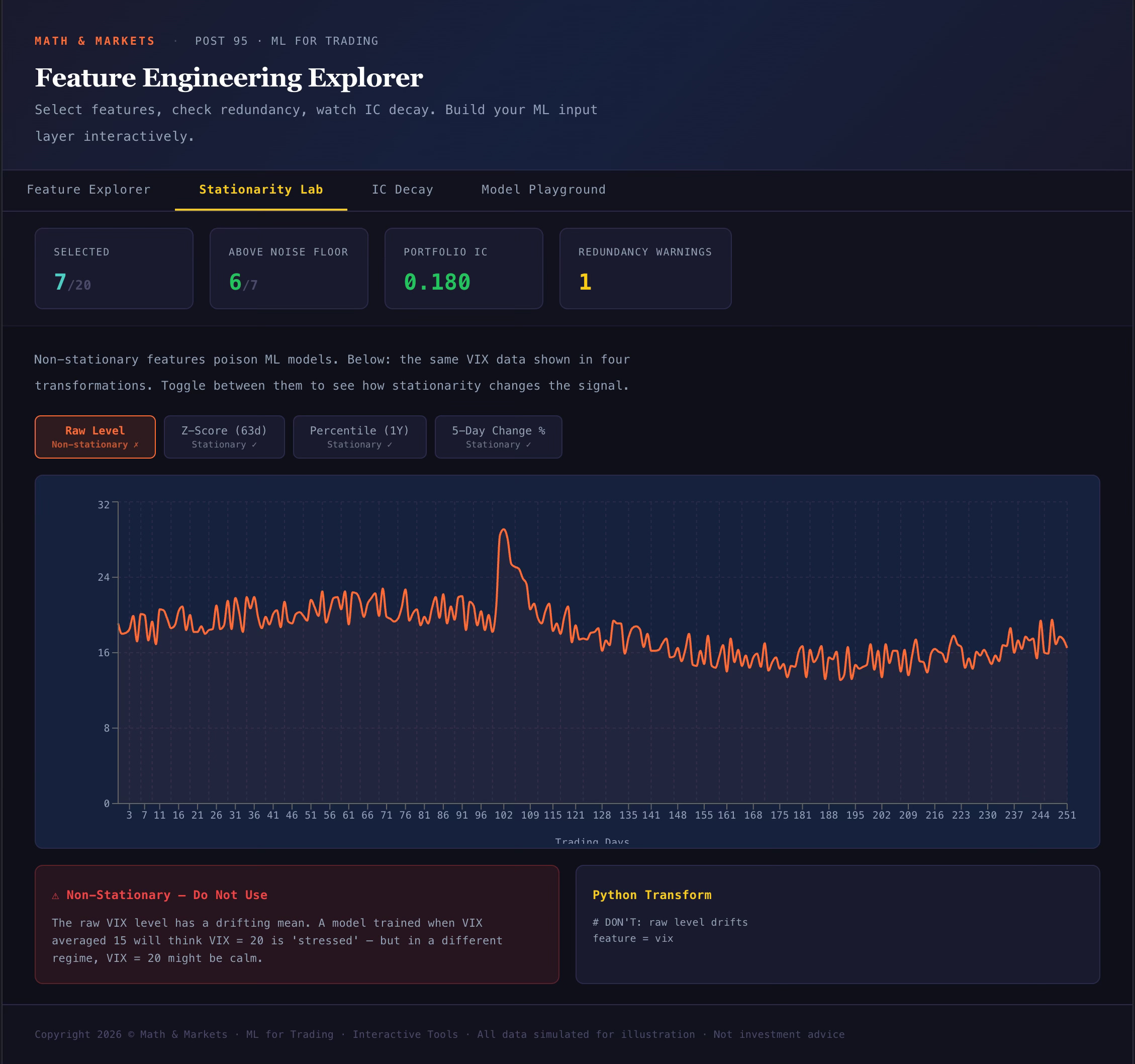
The Stationarity Lab tab shows one feature (VIX) rendered four different ways: raw level, z-score, percentile rank, and rate of change. Toggle between them and notice that the raw level drifts — its mean shifts over time. The other three are stationary. The Python code for each transformation is shown alongside so you can apply the same logic to your own features.
If you take one thing from this tab: never feed a raw level into a model.
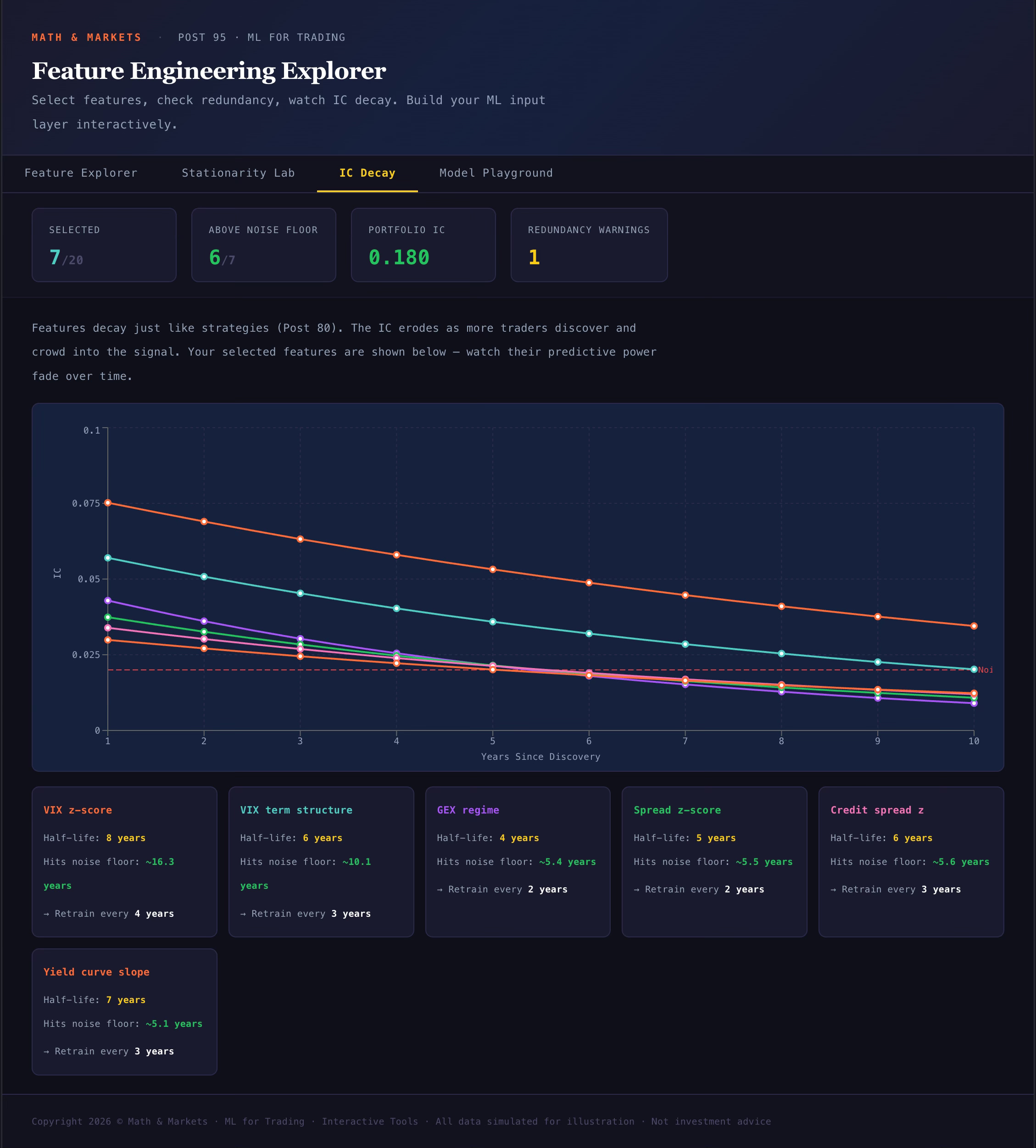
The IC Decay tab shows your selected features losing predictive power over time. Each feature decays at a different rate — VIX z-score holds its IC for roughly 8 years, while OFI proxy drops to the noise floor in about 3. This tab tells you how often your model needs retraining based on the features you’ve chosen.
The Model Playground tab is where you feel overfitting with your hands. Three sliders: number of trees, max depth, and learning rate. As you increase any of them, the in-sample Sharpe climbs — it can hit 1.0, 1.5, even 2.0+. The out-of-sample Sharpe peaks around 200 trees / depth 4 / learning rate 0.05, then collapses. The bar chart shows the gap at every tree count. The verdict text changes from green (”healthy”) to yellow (”moderate overfit”) to red (”your model has memorized the training data”).
Crank the depth to 15 and watch the IS Sharpe hit 2.0+ while OOS drops below 0.3. That’s the chart that should be tattooed on every ML practitioner’s forearm.

Tool 2: SHAP Explorer
ml-shap-explorer.mathandmarkets.com
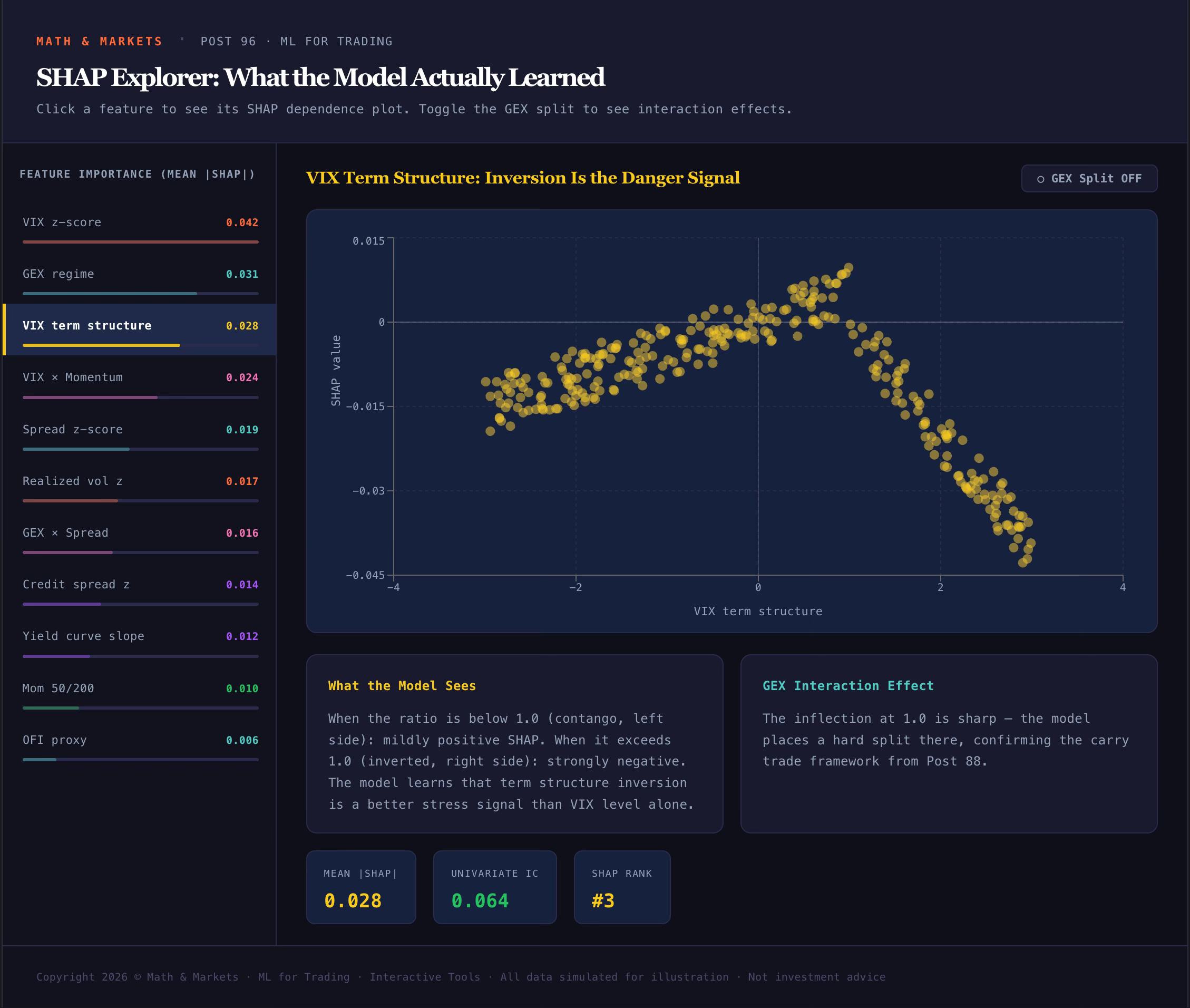
This is the companion to Post 96. It shows what the XGBoost model actually learned — not just which features are important (the bar chart) but how each feature affects the model’s output (the dependence plots).
The sidebar ranks all 11 features by mean |SHAP value|. Click any feature to load its dependence plot in the main panel.
The dependence scatter shows the feature’s value on the x-axis and its SHAP contribution on the y-axis. Each dot is one day. The shape of the cloud tells you the relationship — and the key discovery is that many relationships are non-linear.
Start with VIX z-score. You’ll see a shape that isn’t a straight line. Below zero, SHAP is mildly positive (buy the calm). Between 0 and 2.5, it’s strongly negative (reduce allocation). But above 2.5 — the extreme tail — it bends back up. The model discovered that extreme VIX readings predict mean-reversion, not continuation. That’s the signal my if-else rules missed for 94 posts.
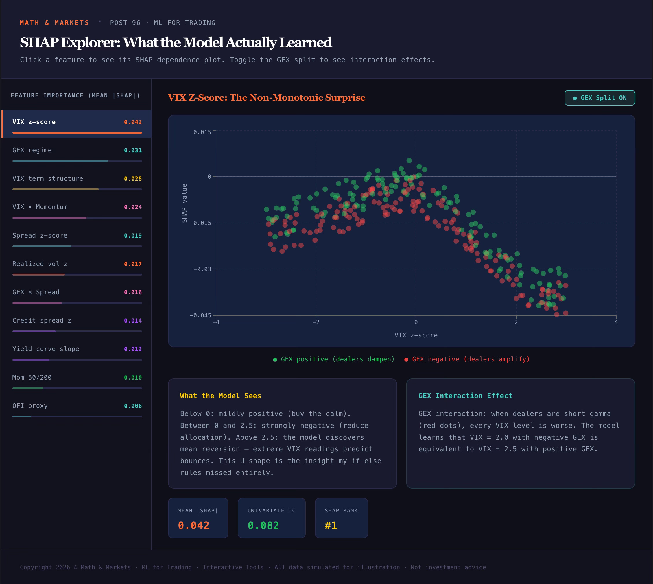
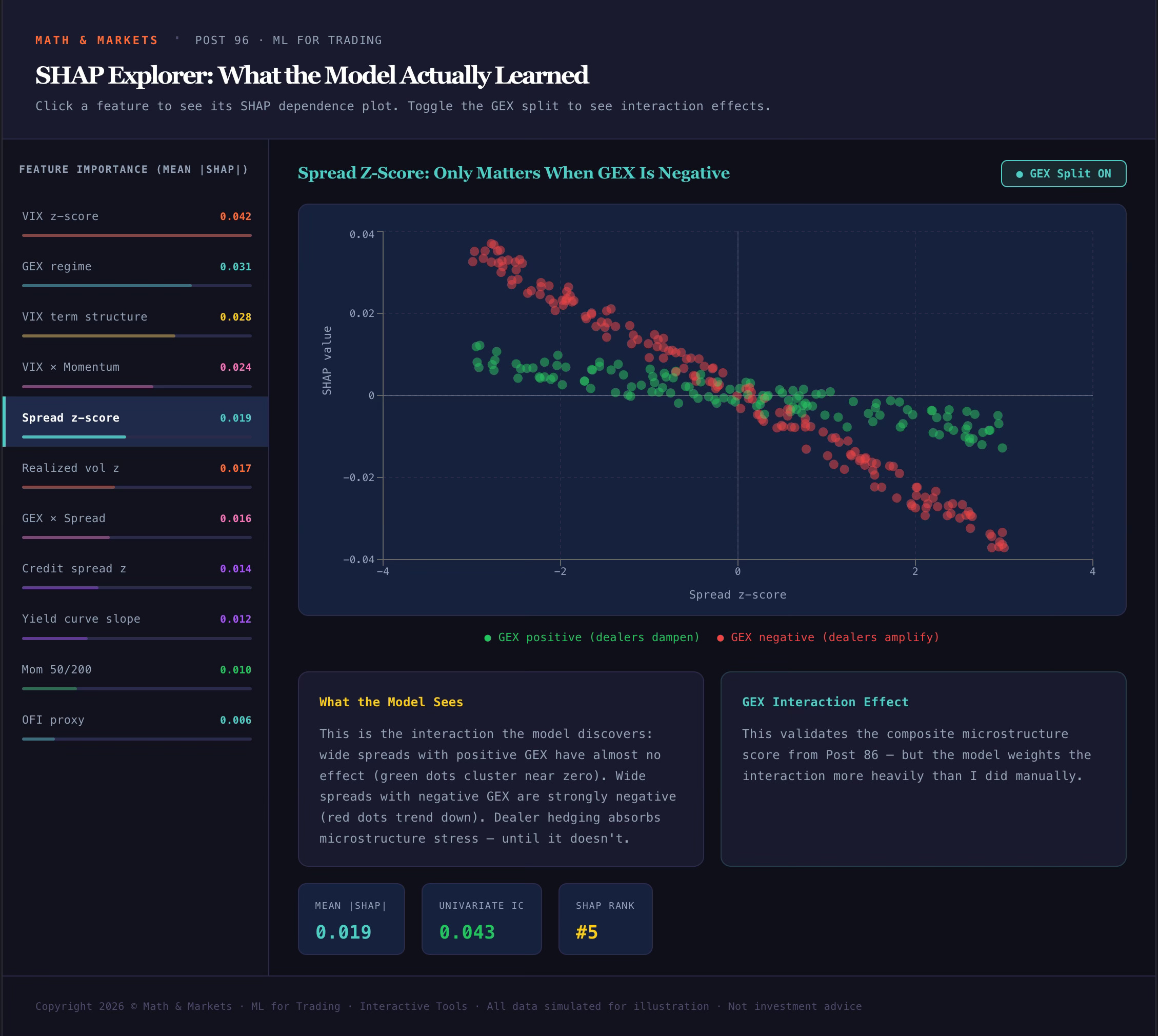
Toggle the GEX split button in the top right. This colors each dot by whether GEX was positive (green) or negative (red) on that day. The two populations separate — negative GEX makes every VIX level worse. The model treats VIX = 2.0 with negative GEX the same as VIX = 2.5 with positive GEX. That’s an interaction effect that linear IC analysis from Post 95 couldn’t detect.
The Spread z-score dependence plot is another one worth examining with GEX split on. Wide spreads with positive GEX have almost no effect — dealer hedging absorbs the microstructure stress. Wide spreads with negative GEX are strongly negative. The interaction is the signal, not the individual feature.
Tool 3: Decision Tree Builder
ml-tree-builder.mathandmarkets.com
This one is a game. Can you build a hand-tuned decision tree that beats XGBoost?
The left panel is your rule builder. Click “+ Add Rule” to create a split. Each rule has four components: a feature (VIX z-score, GEX regime, momentum, etc.), a direction (greater than or less than/equal), a threshold, and an allocation (0-100%). Rules are evaluated top to bottom — the first matching rule wins. Days that don’t match any rule get full allocation.
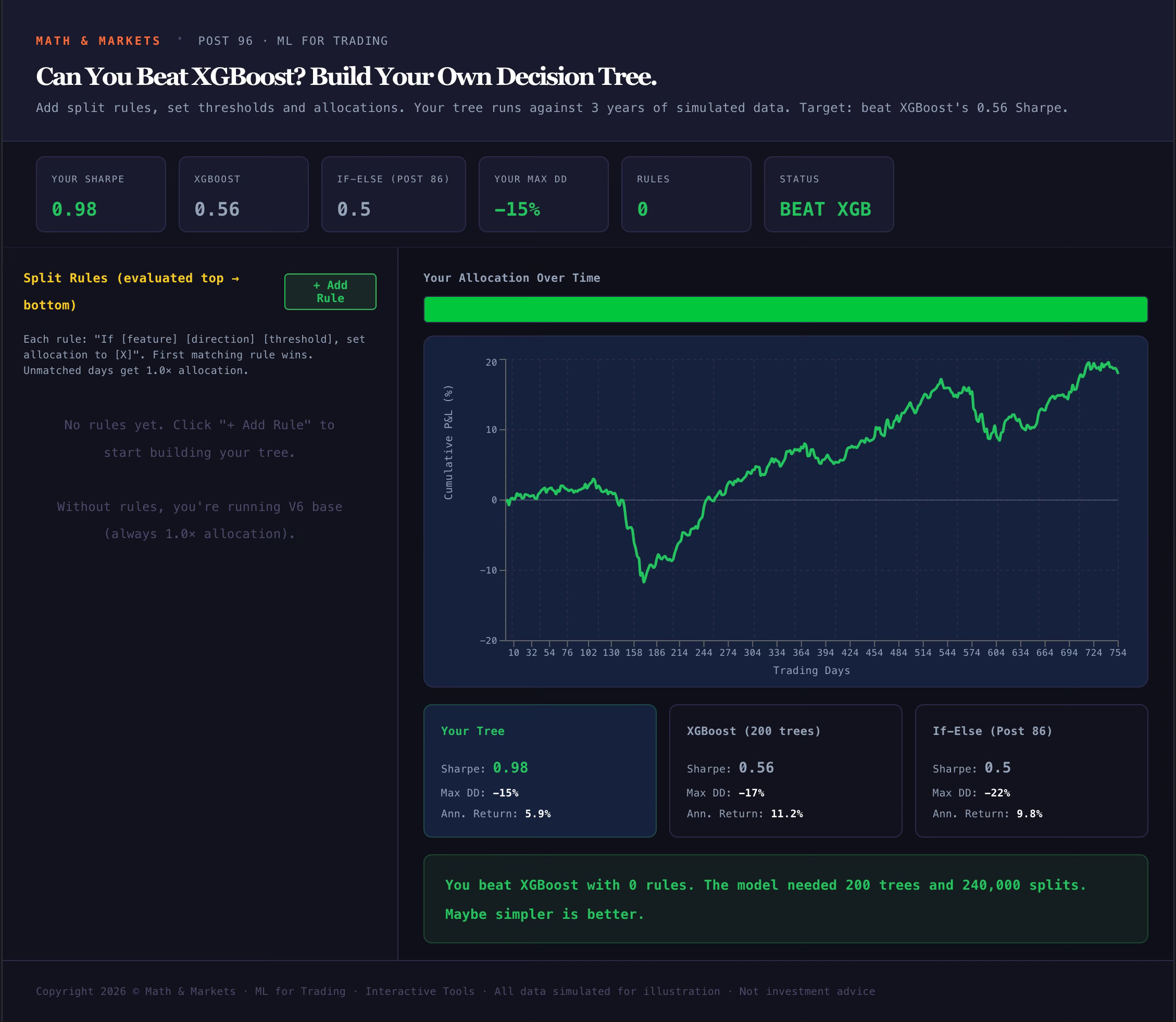
The right panel updates live. You’ll see a heatmap strip showing your allocation over time (green = full, red = minimum), an equity curve comparing your tree to the V6 base, and a results table benchmarking you against XGBoost (Sharpe 0.56) and the if-else rules from Post 86 (Sharpe 0.50).
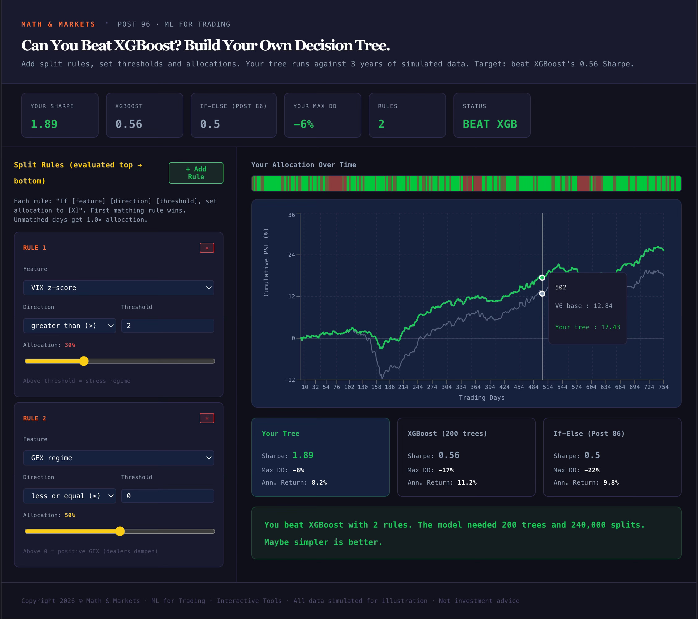
To get started: try adding one rule — VIX z-score > 1.5, allocation 20%. This single rule captures the three stress periods and should push your Sharpe from the base level up toward 0.4-0.5. Then add a second rule for GEX regime <= 0, allocation 50%. This catches days where dealer positioning amplifies moves even when VIX isn’t extreme.
The verdict bar at the bottom tells you where you stand. If you beat XGBoost with fewer rules than it has trees, the verdict will say so — and that’s the point. Sometimes domain expertise in 3 rules beats 200 trees and 240,000 splits.
The hint if you get stuck: the stress periods are around days 130-170, 370-405, and 570-615. The model catches them by combining VIX z-score, momentum direction, and spread width. Try adding a rule that captures negative momentum during high VIX — that’s the regime the model weights most heavily.
What’s Coming Next
These three tools cover Posts 95-96. The next two posts — Post 97 (The Overfitting Minefield) and Post 98 (The V6 ML Layer) — will bring additional interactive components. The walk-forward validation visualizer is in development, and the final post will include a head-to-head simulator where you can compare the ML layer, the if-else rules, and the V6 base across different market regimes.
All tools are at ml-tools-hub.mathandmarkets.com.
Not investment advice. These are simply tools to experiment and play with. Do your own due diligence.
Awesome. The SHAP explorer is my favorite. You need to include a connector between the modules and the main site. There should be an easier way to go from any of the explorers to the main hub.
Wow this is exactly what I need right now. Thank you for taking the time to build this.