From If-Else to XGBoost: Why the Hard Part Isn't the Model

Machine Learning Series Part 1: We Tested 20 ML Features. Only 7 Beat the Noise Floor.

This is part 94 of my series — Building & Scaling Algorithmic Trading Strategies

This begins a 4-part series on machine learning for trading. Part 1: feature engineering. Part 2: tree models for regime classification. Part 3: the overfitting minefield. Part 4: does the ML layer actually help V6?

---

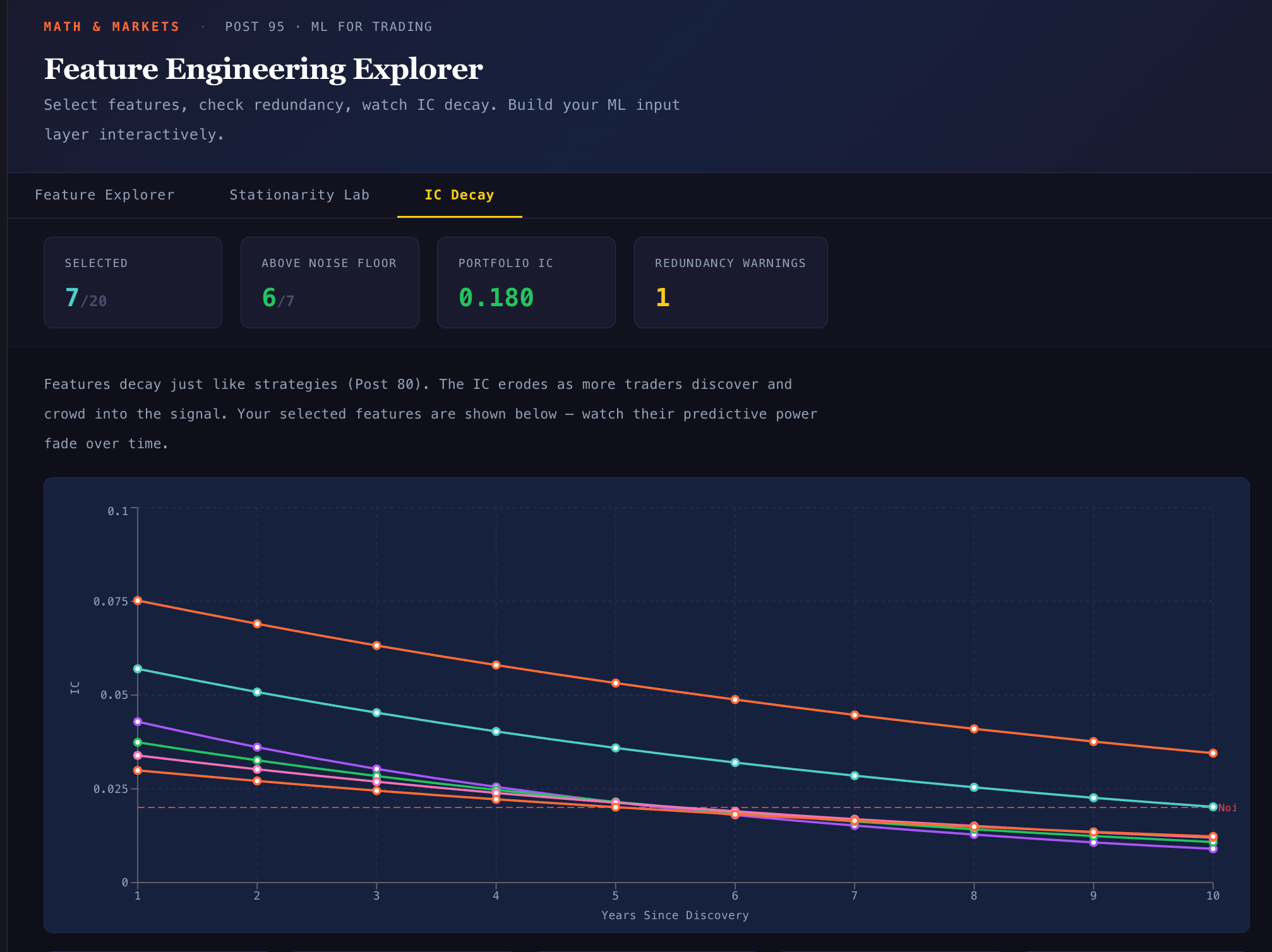
🔧 Interactive tool: ML Feature Engineering Explorer — select from all 20 candidate features, check which ones beat the noise floor, watch their predictive power decay over time, and see the Python transforms for making raw data ML-safe.

---

The Dirty Secret of ML for Trading

Here’s what nobody tells you in the scikit-learn tutorials: the model doesn’t matter.

Not at first. Not until you’ve spent 80% of your time on the input. A random forest trained on good features will crush a transformer trained on garbage. A logistic regression with the right 8 features will beat a neural network with 200 noisy ones. The model learns patterns in whatever you feed it. If you feed it noise, it learns noise.

This post is about the 80% — feature engineering. Specifically: how to convert 93 posts of trading signals, macroeconomic indicators, and microstructure data into a clean, stationary, non-redundant feature set that a model can actually learn from.

---

The Feature Taxonomy

Over the last 15 posts (Parts 80-94), we built signals across five categories. Here they all are:

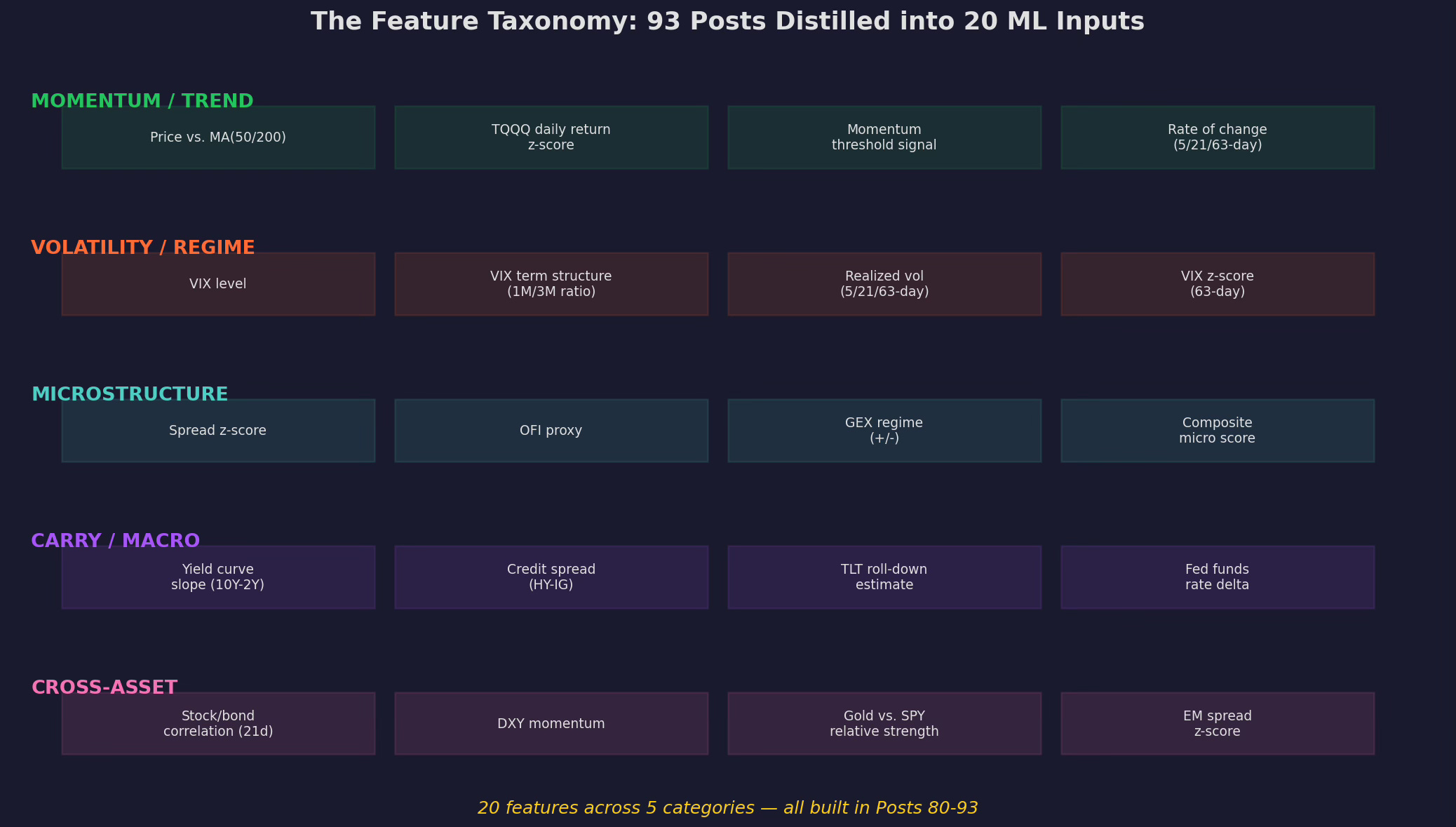
Twenty candidate features organized by category. Momentum/trend features capture directional persistence. Volatility/regime features capture market stress. Microstructure features capture order flow and dealer positioning. Carry/macro features capture the yield environment. Cross-asset features capture inter-market relationships.

Each of these features was developed and discussed in a specific post. They’re not random — they have theoretical grounding and empirical motivation. But that doesn’t mean they all belong in an ML model. Many are redundant, some are non-stationary, and a few might be pure noise in a multivariate context.

The job of feature engineering is to separate the signal from the noise, the unique from the redundant, and the stationary from the drifting.

---

Problem 1: Redundancy

The first thing you notice when you stack these features into a correlation matrix:

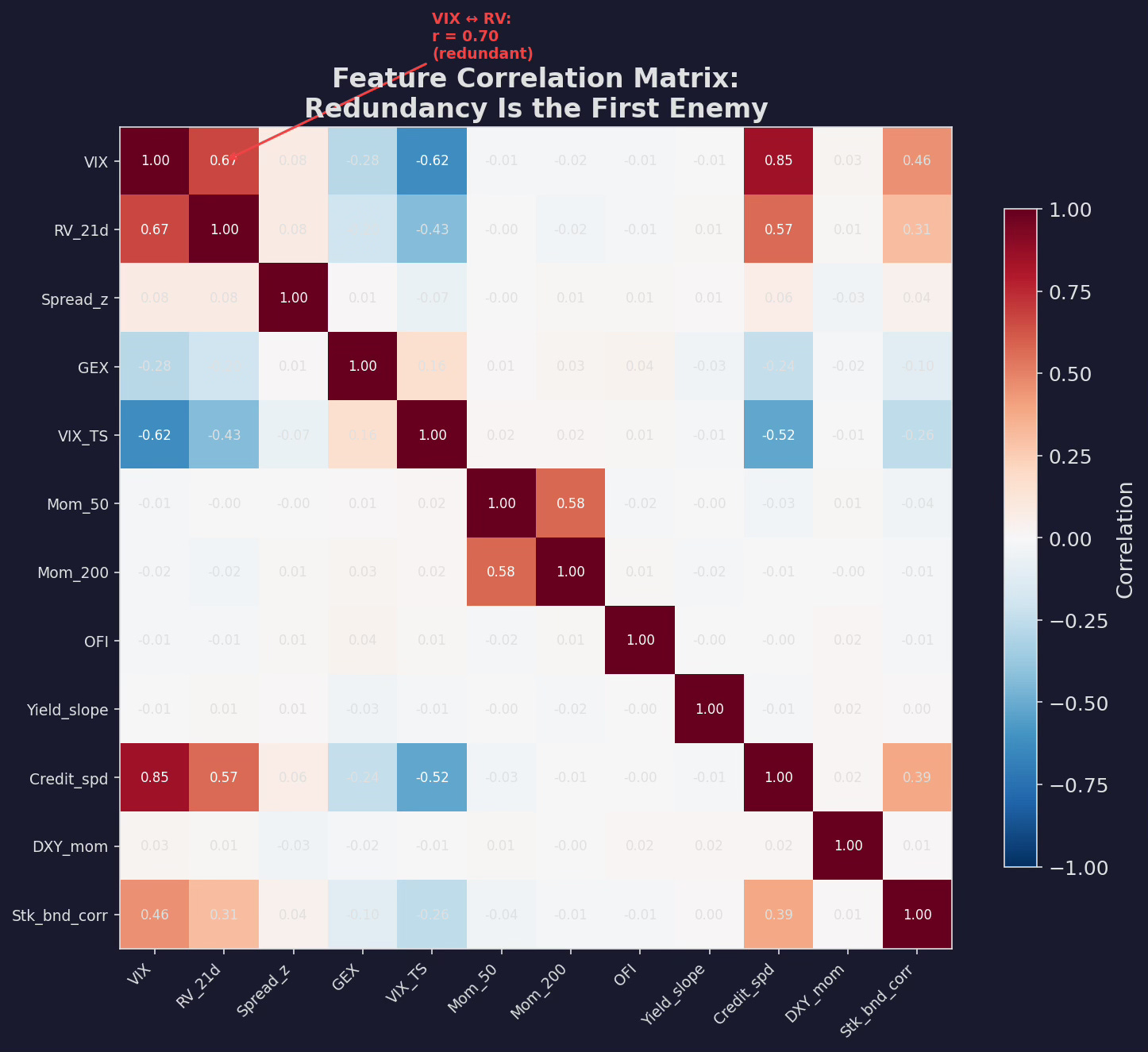
Pairwise correlations across 12 features. VIX and 21-day realized vol are 70% correlated — they’re measuring the same thing. 50-day and 200-day momentum have 50% overlap. Credit spreads and VIX are 40% correlated. Feeding all of these into a model gives you multicollinearity — the model can’t separate the contribution of each feature.

The fix is straightforward: for each pair with |r| > 0.7, drop one. The decision of which to drop is domain-driven:

Between VIX and realized vol, keep VIX — it’s forward-looking (implied) while RV is backward-looking (realized). The forward-looking version is more useful for predicting future returns.

Between Mom(50) and Mom(200), keep the ratio (50/200) rather than either level — the crossover signal carries the information of both in a single feature.

Between credit spreads and VIX, keep both — the correlation is moderate (0.4) and they capture different aspects of risk (credit vs. equity volatility). But if forced to choose, credit spreads add incremental information that VIX doesn’t capture.

After the correlation filter: 20 candidates → ~14 features.

---

Problem 2: Stationarity

This is where most retail ML projects fail silently.

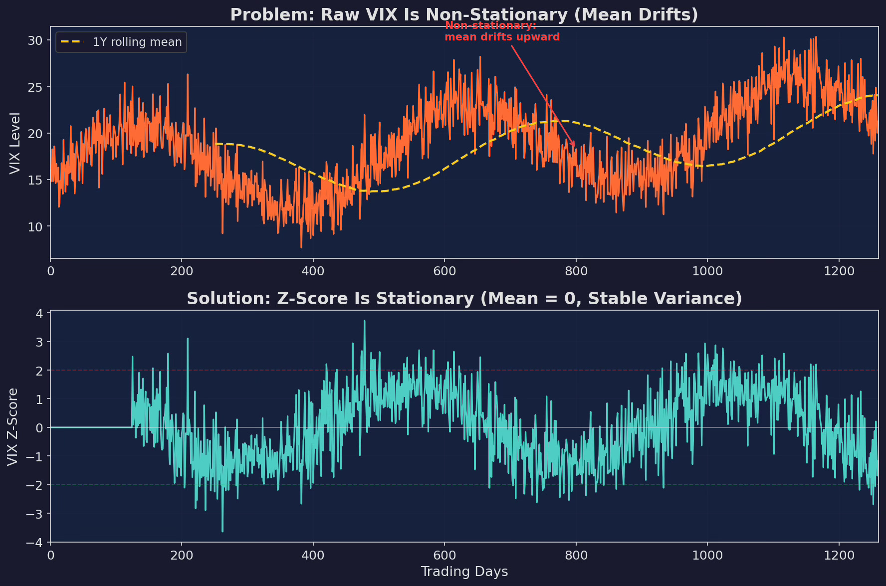
Top: raw VIX level over 5 years. The mean drifts upward — a model trained on the first 2 years would learn “VIX above 18 is high” but by year 5, VIX is regularly above 20 even in calm markets. Bottom: VIX z-score (126-day) is stationary — mean zero, stable variance. A z-score of +2 means the same thing in year 1 and year 5.

Non-stationary features poison ML models because the relationship between feature and target shifts over time. A model trained in a low-VIX era will have learned that VIX = 20 is “stressed.” Deploy it in a high-VIX era where VIX = 20 is “calm,” and it will persistently overestimate risk.

The rule: never feed a raw level into a model. Always transform to a stationary representation.

Four transformations, from simplest to most robust:

# 1. Z-score (most common)
z = (x - x.rolling(63).mean()) / x.rolling(63).std()

# 2. Percentile rank (non-parametric, handles skew)
pct = x.rolling(252).apply(lambda w: (w.iloc[-1] > w).mean())

# 3. Rate of change (captures dynamics)
roc = x.pct_change(21)

# 4. Binary regime (simplest, most robust)
regime = (x > x.rolling(126).median()).astype(int)

Which to use? Z-scores work for normally distributed features (vol, spreads). Percentile ranks work for everything but lose granularity. Rates of change work for trending features (momentum, yield curve). Binary regimes sacrifice precision for robustness — which matters when the model will see out-of-sample data that looks nothing like the training set.

---

Problem 3: Individual Features Are Weak

Here’s the uncomfortable truth about financial prediction: most features have an information coefficient (IC) — the rank correlation between the feature today and the return over the next week — of approximately 0.02 to 0.08.

This is a lesson I’ve had to learn over and over again, but I still keep repeating the same mistake.

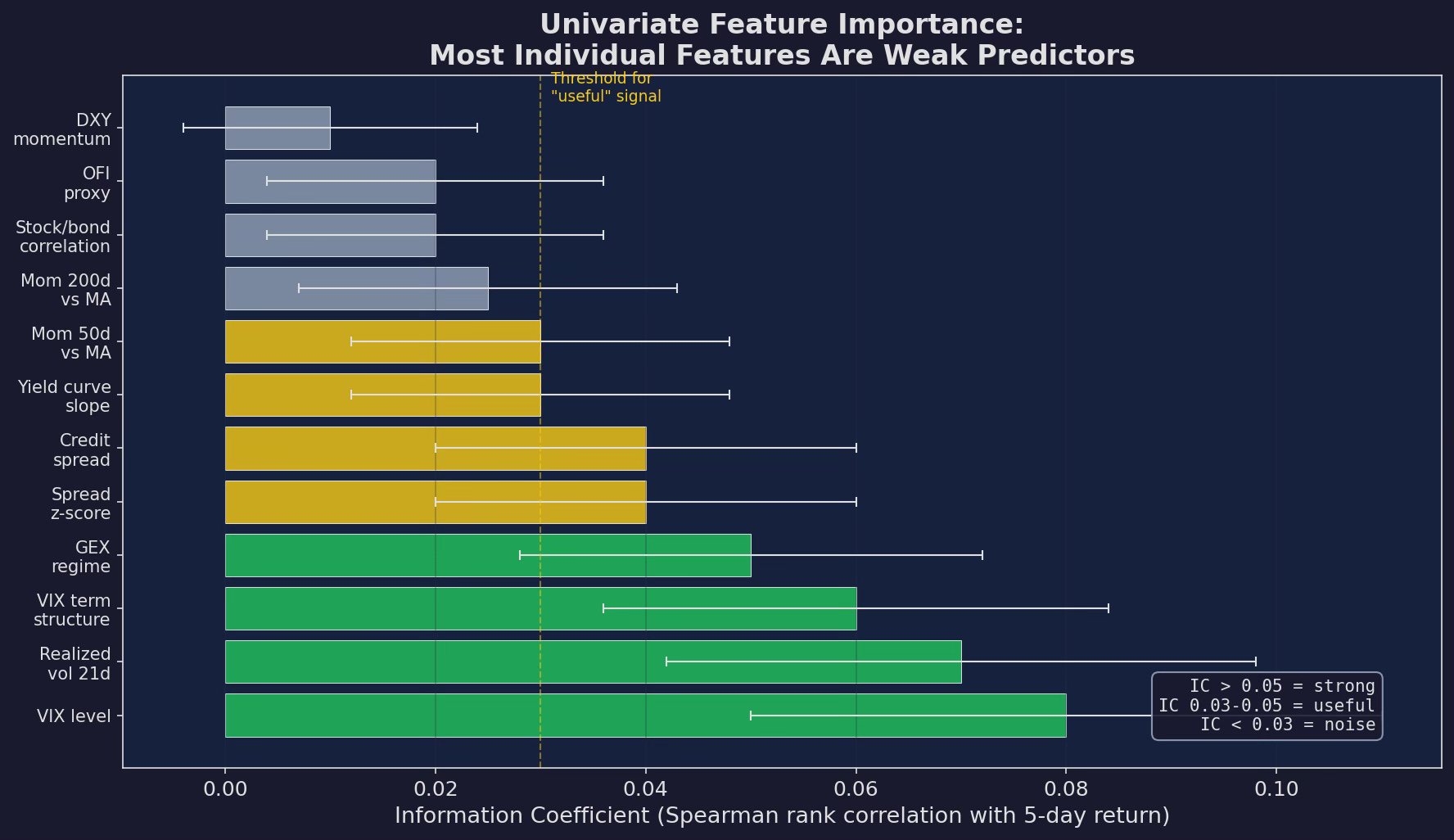
Univariate IC for each candidate feature. VIX level is the strongest predictor at IC ≈ 0.08 — which means it explains roughly 0.6% of the variance in next-week returns. Most features are below 0.05. Some are below 0.02, which is indistinguishable from noise.

For context: an IC of 0.05 means that if you ranked all days by the feature value and sorted them into quintiles, the top quintile would outperform the bottom quintile by roughly 2-3% annualized. That’s meaningful for a systematic strategy but invisible on any individual trade.

This is why ML helps: individual features are weak, but their combination can be strong. If VIX, term structure, GEX, and spread z-score each independently predict returns at IC ≈ 0.05 and they capture different dimensions of risk, a model that combines them might achieve IC ≈ 0.10-0.12 through the aggregation of weakly correlated weak predictors.

This is the “wisdom of crowds” principle applied to features. No single expert (feature) is very good. But the committee (model) can be substantially better than any individual member, provided the members aren’t all saying the same thing (low inter-feature correlation).

---

The Transformation Toolkit

One raw feature can produce multiple transformed features. The question is which transformations capture useful information:

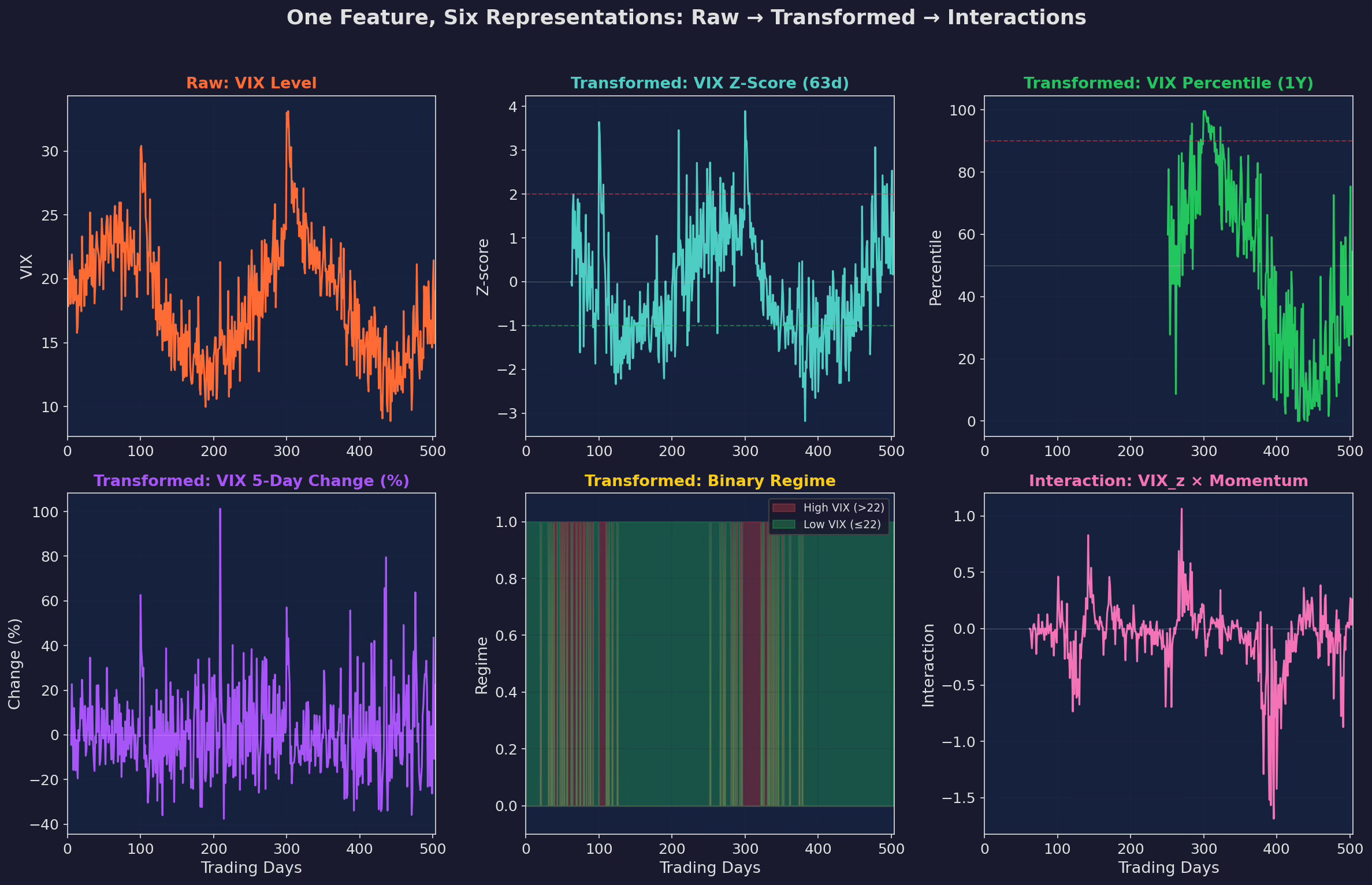
Six representations of a single input (VIX). Raw level (non-stationary, avoid). Z-score (stationary, captures deviation from recent norm). Percentile rank (robust, captures relative positioning). Rate of change (captures acceleration/deceleration). Binary regime (simplest, most robust). Interaction term (VIX_z × momentum, captures non-linear dependencies).

Interaction Features

Interaction features are where domain expertise meets statistical power. Two features that are individually weak can be jointly powerful if their interaction captures a meaningful dynamic:

VIX_z × Momentum: High VIX with negative momentum = crash regime. High VIX with positive momentum = recovery bounce. The interaction separates these two regimes that VIX alone cannot distinguish.

GEX × Spread_z: Negative GEX with wide spreads = maximum microstructure stress. Negative GEX with normal spreads = moderate stress. The interaction captures severity better than either feature alone.

Yield_slope × Credit_spread: Steep curve with tight credit = risk-on carry environment. Steep curve with wide credit = economic distress. The interaction disambiguates.

The danger of interactions: every pair you add is a new feature that the model can overfit to. With 14 base features, you have 91 possible interactions. Adding all of them is a recipe for overfitting. Add only the interactions that have clear economic interpretation.

---

The Selection Pipeline

Putting it all together:

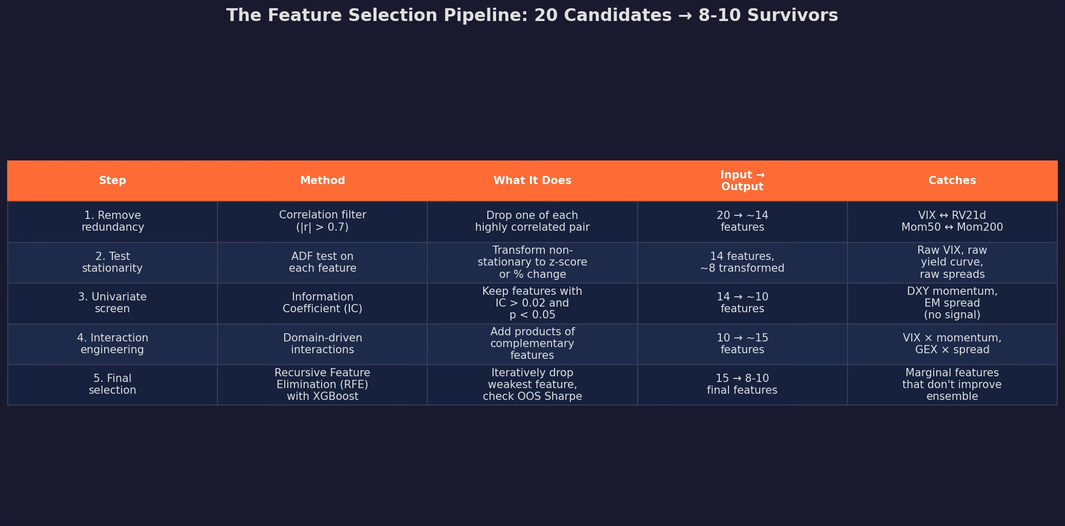
Starting with 20 candidates, the pipeline produces 8-10 final features through five stages. Each stage has a clear purpose and a clear rule for what survives.

The output of this pipeline is the feature matrix X that gets fed into the model in Part 2. I’d say that the pipeline is not optional — skipping any stage (especially stationarity testing and redundancy removal) will produce a model that looks great in-sample and falls apart out-of-sample.

---

The Half-Life of Features

One more complication: features decay, just like strategies (Post 80).

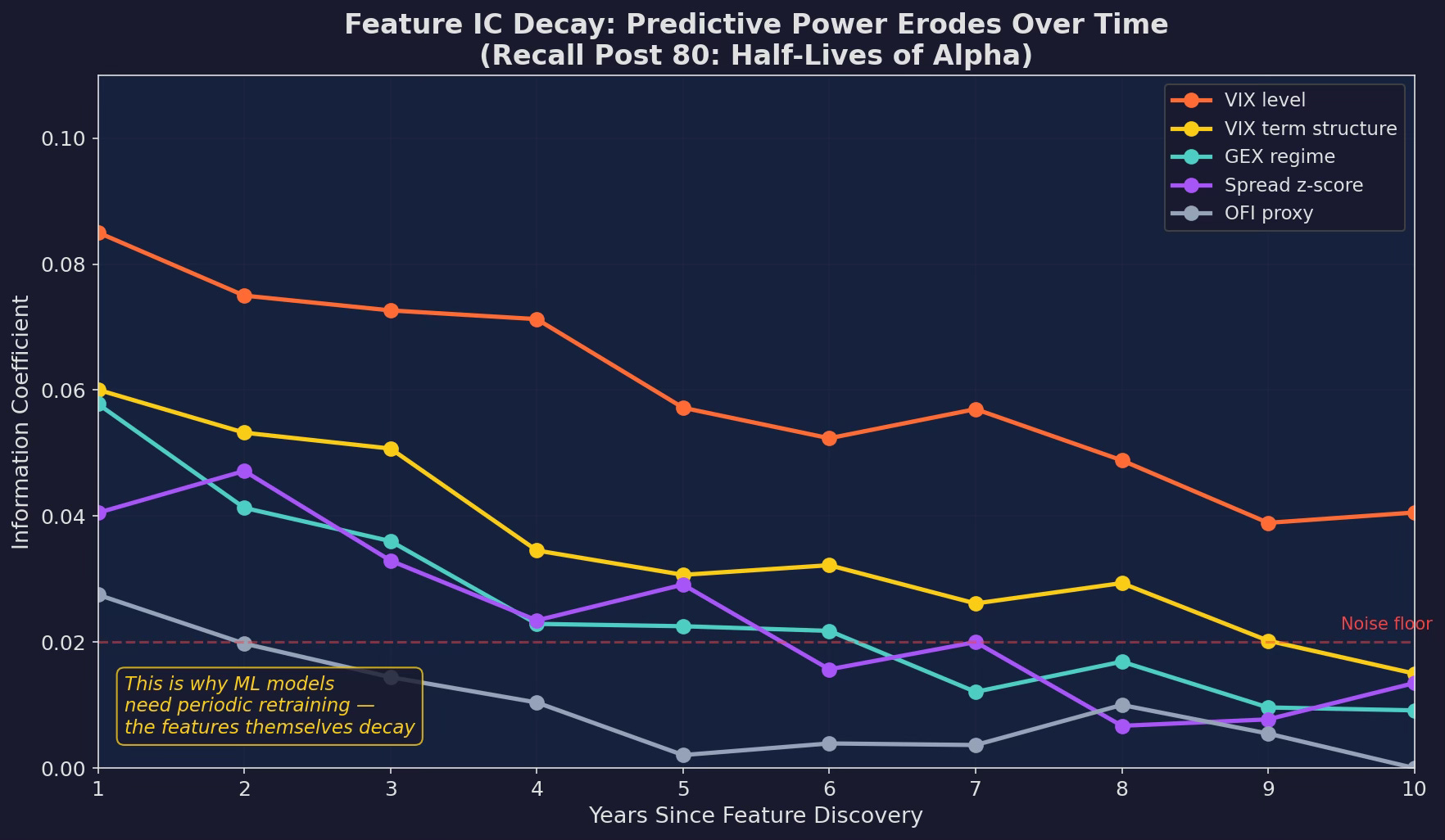
Information coefficient over time for five features. VIX level maintains predictive power longest (structural, rooted in risk aversion). OFI proxy decays fastest (microstructure signals get crowded). GEX regime sits in between. All features trend toward the noise floor of IC ≈ 0.02 eventually.

This connects directly to the Strategy Decay series. The alpha in a feature comes from an informational edge. As more people learn about and trade on GEX signals (thanks partly to the popularization by SpotGamma and others), the feature’s predictive power decays. VIX decays more slowly because it’s structural — risk aversion doesn’t get arbitraged away.

The implication for ML: your model needs periodic retraining not just because the model degrades, but because the features themselves degrade. A model trained in 2020 using GEX as a strong feature might find that GEX has an IC of 0.01 by 2025 — below the noise floor. The model needs to downweight or drop it.

This is the feature engineering → model training → retraining feedback loop. We’ll build the retraining framework in Part 3.

---

What the Feature Matrix Looks Like

After the full pipeline, here’s the concrete feature matrix for V6:

features = {
    # Volatility / Regime (3 features)
    'vix_z':        vix_zscore_63d,
    'vix_ts':       vix_1m_div_3m,
    'rv_z':         realized_vol_z_63d,  # keep if corr with vix_z < 0.7
    
    # Microstructure (2 features)
    'gex_regime':   gex_binary,           # +1 / -1
    'spread_z':     spread_zscore_21d,
    
    # Momentum (2 features)
    'mom_ratio':    ma50_div_ma200,
    'mom_roc':      price_roc_21d,
    
    # Carry / Macro (2 features)
    'yield_slope_z': yield_10y2y_zscore,
    'credit_z':     hy_ig_spread_zscore,
    
    # Interactions (2 features)
    'vix_x_mom':    vix_z * mom_roc,
    'gex_x_spread': gex_regime * spread_z,
}

# Target: next 5-day V6 excess return (over SPY)
target = v6_return_5d - spy_return_5d

Eleven features that are clean, stationary, non-redundant, with domain-driven interactions. This is what gets fed into Part 2’s tree models.

---

Up Next

Part 2: Tree Models for Regime Classification — Random forests, XGBoost, and why tree-based models are the right tool for this problem. We’ll train, validate, and stress-test the models using the feature matrix we just built.

---

Remember: Alpha is never guaranteed. And the backtest is a liar until proven otherwise.

These posts are about methodology, not recommendations. If you find errors in my math, let me know — I’ve built an entire series around discovering my own mistakes, so one more won’t hurt.

The material presented in Math & Markets is for informational purposes only. It does not constitute investment or financial advice.

---