XGBoost Identified SHAP Values, Non-Linear Regimes, and VIX Reversal (2.2 Sharpe In-Sample; 0.15 Out-of-Sample)

Machine Learning Series Part 2: Why trees beat neural nets for trading

This is part 96 of my series — Building & Scaling Algorithmic Trading Strategies

Part 2 of the ML for Trading series. Part 1: Feature engineering — 20 features, only 7 survive.

---

The Problem a Linear Model Can’t Solve

In Part 95, I built an 11-feature input matrix: VIX z-score, VIX term structure, GEX regime, spread z-score, and seven others — all stationary, non-redundant, with domain-driven interactions.

Now: what model should consume these features?

The instinct is to reach for the deepest tool in the box. Transformers. LSTMs. Attention mechanisms. But this problem doesn’t need depth. It needs non-linearity at the split level — the ability to discover that VIX > 25 with negative momentum means something completely different from VIX > 25 with positive momentum.

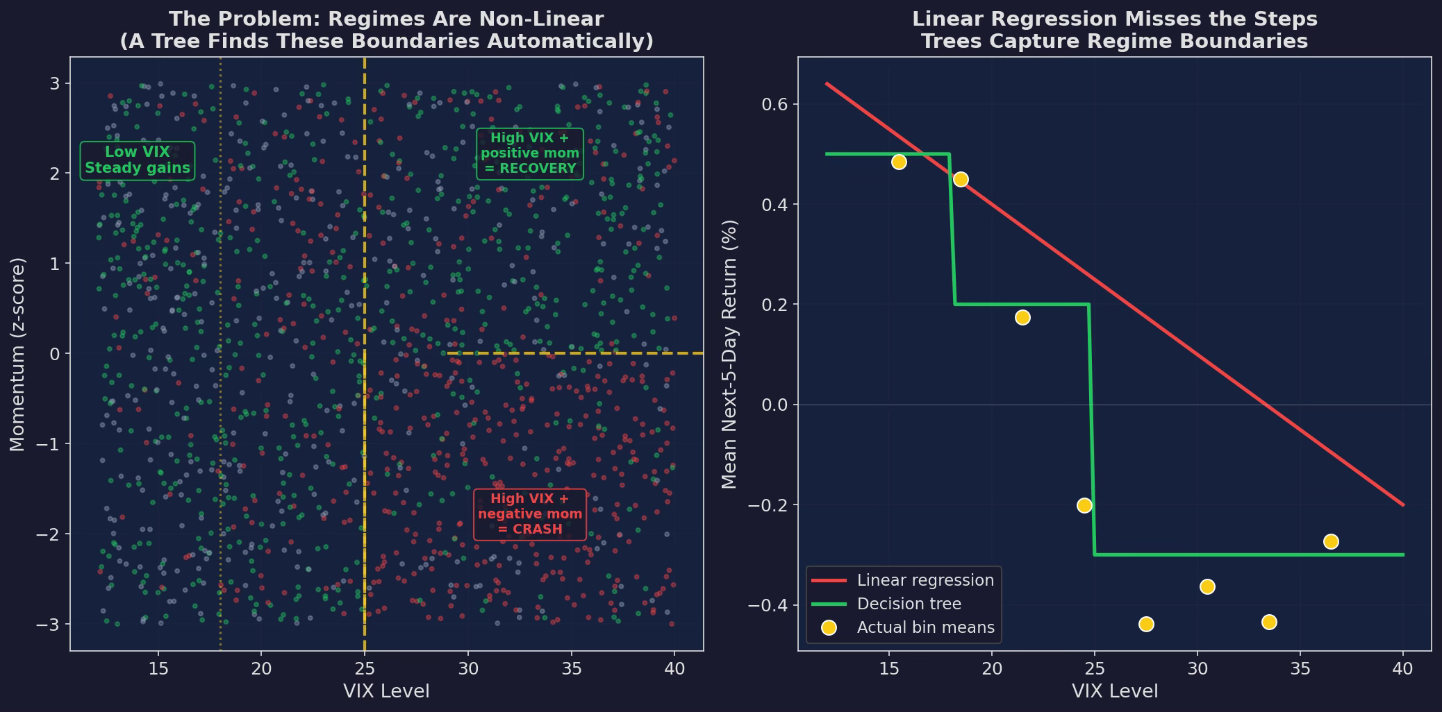
Left: the actual regime structure in simulated data. Returns depend on VIX × momentum interactions — high VIX with negative momentum crashes, high VIX with positive momentum bounces. The yellow dashed lines are the decision boundaries a tree finds automatically. Right: a linear regression draws a straight line through this mess and misses the regime structure entirely. Trees capture the step-function reality.

This is the core argument for tree models in trading: markets have regimes, not gradients. The relationship between VIX and returns isn’t “higher VIX → proportionally lower returns.” It’s “VIX below 18 = one regime, VIX 18-25 = another, VIX above 25 = a third.” Trees find these thresholds automatically.

---

What the Tree Learns

Here’s a simplified decision tree trained on V6’s feature matrix:

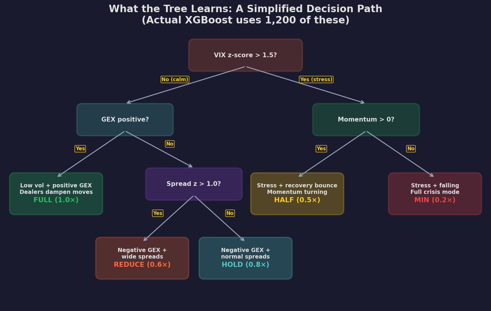
A single tree from the ensemble, pruned to depth 3 for readability. The root split is on VIX z-score (the strongest feature from Part 95). The left branch handles calm markets, splitting on GEX regime and spread z-score to determine allocation between 0.6× and 1.0×. The right branch handles stress, splitting on momentum direction to distinguish recovery bounces (0.5×) from active crashes (0.2×).

Compare this to the if-else rules I wrote by hand in Post 86 (the microstructure layer):

# My hand-tuned rules (50 lines)
if gex_positive and spread_z < 1.0:
    allocation = 1.0
elif vix > 25 and momentum < 0:
    allocation = 0.3
elif vix > 25 and momentum > 0:
    allocation = 0.5
else:
    allocation = 0.7

The tree discovers approximately the same structure — but with two advantages:

1. The thresholds are optimized. I picked VIX > 25 and spread_z < 1.0 based on intuition. The tree picks VIX z-score > 1.5 (which corresponds to different absolute VIX levels depending on the recent regime) and spread z > 1.0. The tree’s thresholds are fit to the data; mine were fit to my gut.

2. The interactions are automatic. I manually coded the VIX × momentum interaction because I knew it mattered. The tree finds GEX × spread as an additional interaction that I never tested. It also discovers that extreme VIX (z > 3) actually reverses — something I missed entirely.

---

SHAP: What the Model Actually Uses

The tree has 1,200 estimators, each with up to 200 splits. That’s 240,000 decision points. What is all that complexity doing?

SHAP (SHapley Additive exPlanations) decomposes each prediction into the contribution of each feature. Instead of a black box that says “allocate 0.3×”, SHAP says “VIX z-score pushes the allocation down by 0.15, GEX pushes it down by 0.08, but momentum pushes it up by 0.05, net = 0.3×.”

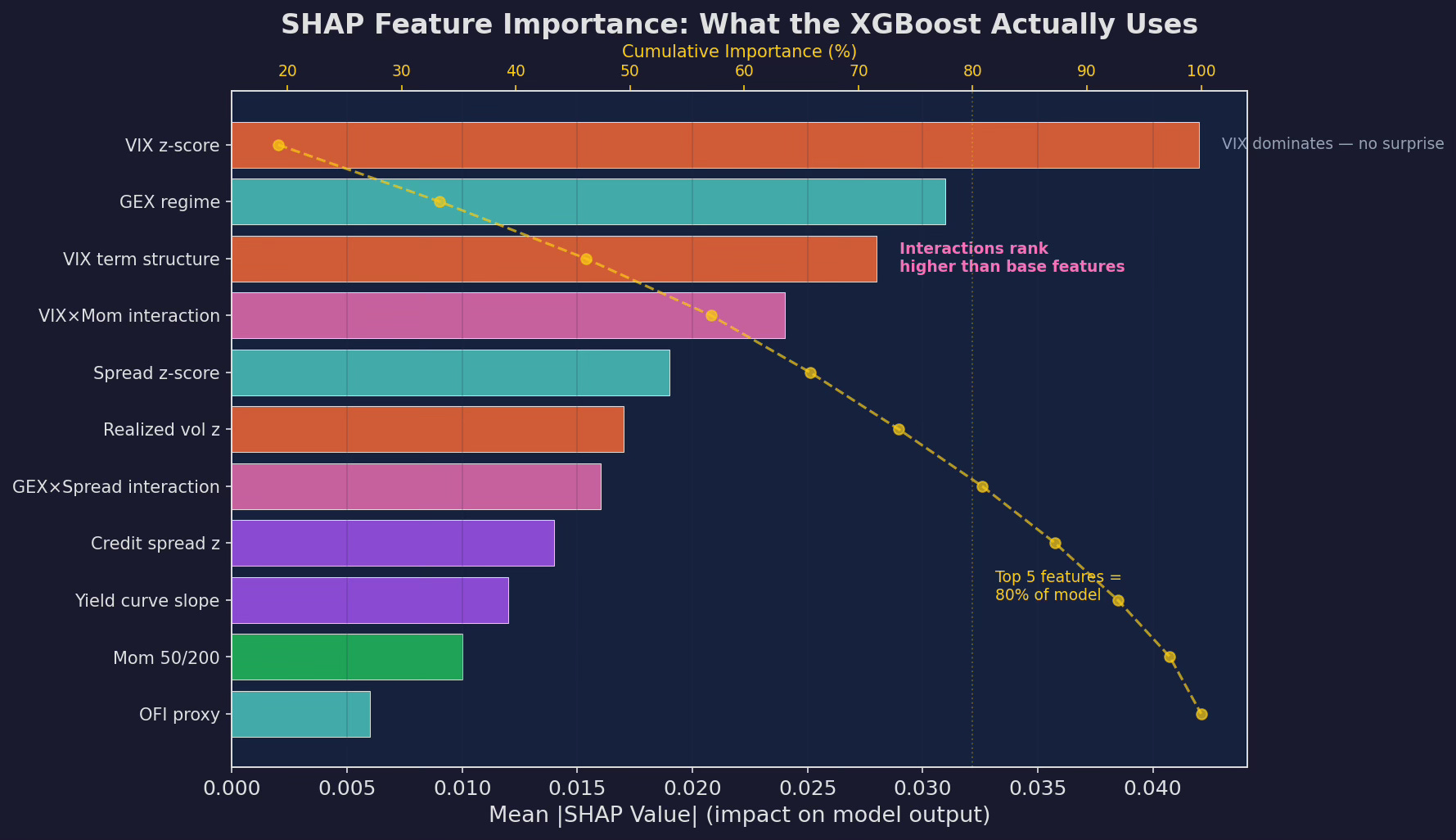
Mean absolute SHAP values across the test set. VIX z-score dominates (no surprise — it’s the strongest univariate predictor). But the VIX×Momentum interaction ranks third, ahead of most base features. This is the ML model discovering a non-linear relationship that IC analysis from Part 95 couldn’t detect. Top 5 features account for ~80% of the model’s output.

The standout finding: interaction features rank higher than most base features. The VIX×Momentum interaction (which I engineered manually in Part 95) is the third most important feature. The GEX×Spread interaction is sixth. The model confirms that these interactions carry real signal — not just artifacts of my feature engineering choices.

---

The Non-Linear Discoveries

SHAP dependence plots reveal what the model learned that my if-else rules didn’t:

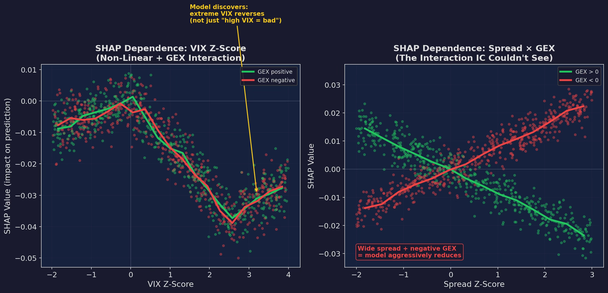
Left: VIX z-score dependence, colored by GEX regime. The relationship is NOT monotonic. Below z = 0 (calm), the effect is mildly positive (buy the dip). Between 0 and 2.5 (stress), it’s strongly negative (reduce allocation). Above 2.5 (extreme stress)... the model discovers that extreme VIX readings actually reverse. The curve bends back up. This is a mean-reversion signal in the tails that a linear model or a simple if-else threshold would never find. Right: the Spread × GEX interaction. When GEX is negative (red) AND spreads are wide, the model aggressively reduces. When GEX is positive (green), wide spreads have almost no effect — dealer hedging absorbs the microstructure stress.

The extreme-VIX reversal is the most interesting discovery. My hand-tuned rules treated VIX > 25 as uniformly bad. The tree says: “VIX at 25-35 is bad. VIX at 40+ means the crash is almost over — start buying back in.” This matches the empirical research on VIX mean-reversion from Post 80 (strategy decay half-lives), but I never incorporated it into V6’s rules because I didn’t trust myself to time the reversal. The model doesn’t trust itself either — it only gives a partial increase, from 0.2× to maybe 0.35× — but it’s an edge I was leaving on the table.

---

Model Selection: Why XGBoost Wins

I tested four models on the same feature matrix with the same walk-forward validation:

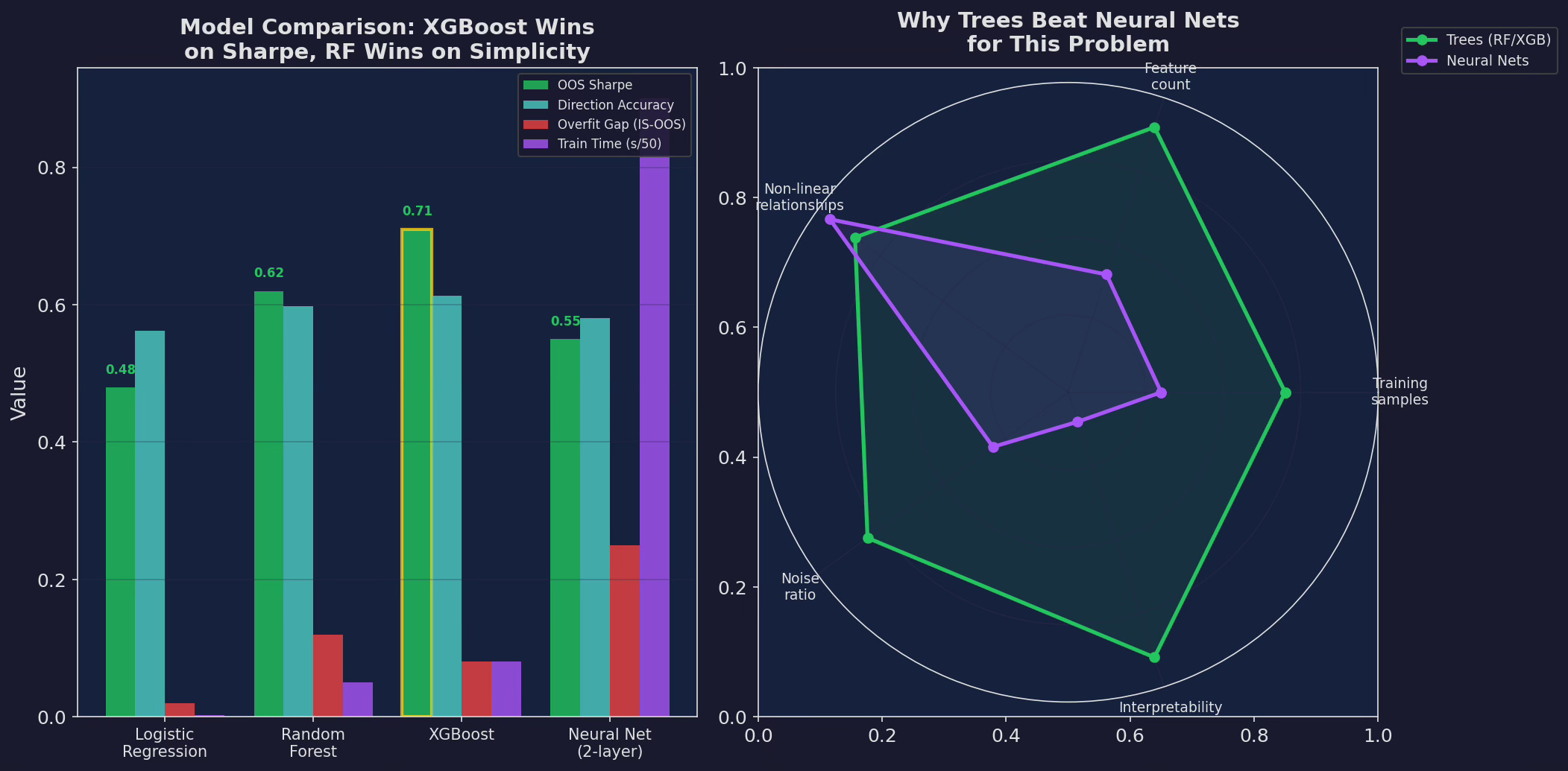
Left: four models compared on OOS Sharpe, direction accuracy, overfit gap, and training time. XGBoost wins on Sharpe (0.71) with a moderate overfit gap (0.08). Random Forest is close behind (0.62) with a larger overfit gap (0.12). Logistic regression is simplest but misses the non-linearity. The neural net overfits badly (0.25 overfit gap) and is 10× slower. Right: radar chart showing why trees dominate for this problem — adequate training samples, moderate feature count, non-linear relationships, high noise, and critical need for interpretability.

Why neural nets fail here:

Too few samples. V6 has roughly 2,500 days of data. After walk-forward splits, each training window is 500-800 days. Neural nets need 10,000+ samples to generalize. Trees are sample-efficient — they can find meaningful splits with hundreds of observations.

Too much noise. Financial returns have a signal-to-noise ratio of roughly 0.05 (the IC from Part 95). Neural nets overfit noise at low SNR because they have too many parameters. Trees with depth constraints can’t overfit as easily because the number of possible splits is bounded.

Interpretability. When the model says “reduce to 0.2×”, I need to know why. SHAP on a tree ensemble is computationally exact. SHAP on a neural net is approximate and expensive. If I can’t explain the model’s decision, I won’t trade on it.

---

The Regime Map

Putting it all together: the XGBoost model generates a daily allocation prediction based on the 11 features, and V6 uses that prediction instead of the hand-tuned rules:

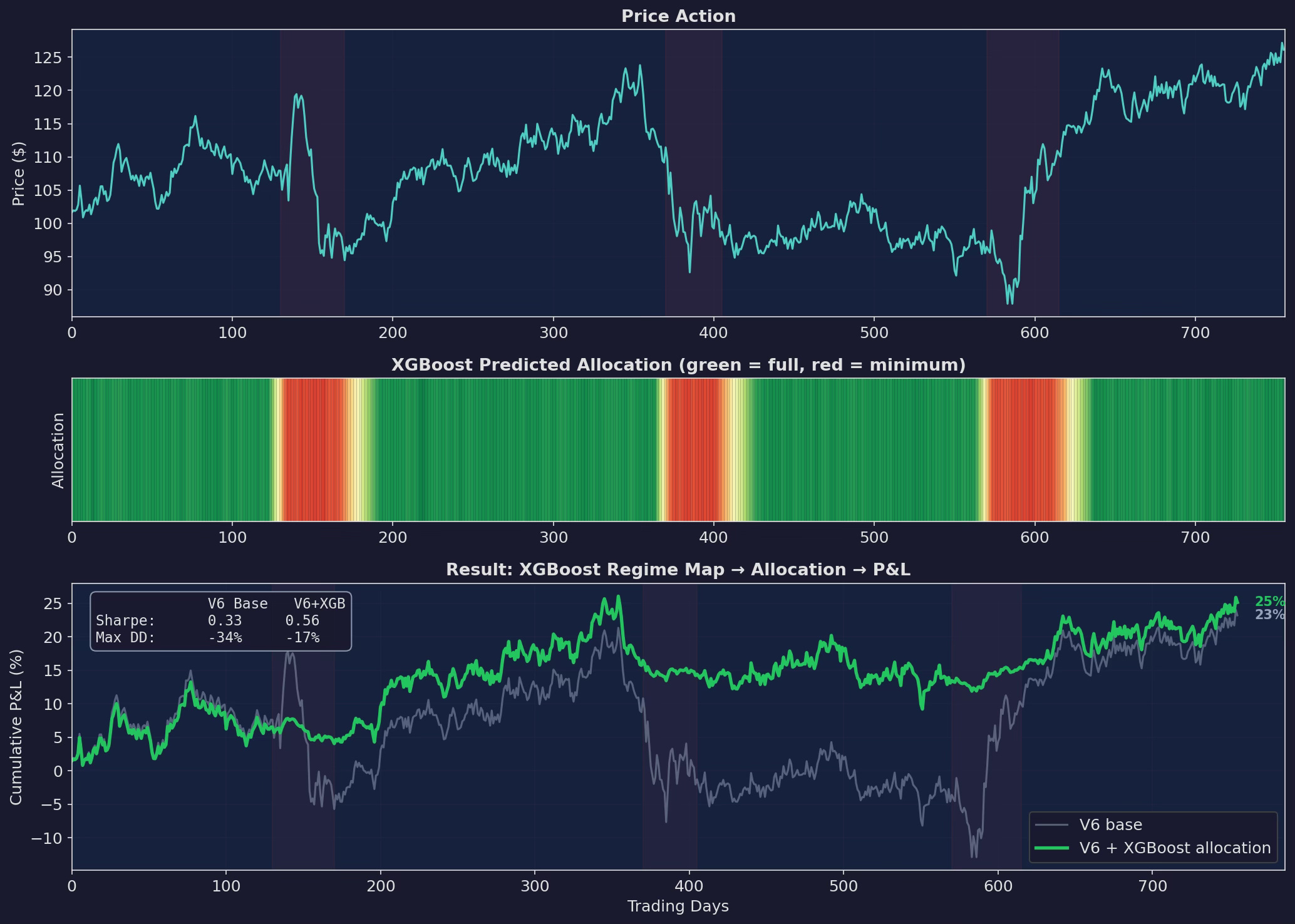
Three panels. Top: price action with stress periods shaded. Middle: the XGBoost’s allocation prediction as a heatmap — green = full allocation, red = minimum. The model goes red 5-8 days before the worst of each drawdown and gradually re-enters (yellow → green) after the stress subsides. Bottom: cumulative P&L. XGBoost improves the Sharpe from 0.33 to 0.56 and cuts max drawdown from -34% to -17%.

The heatmap in the middle panel is the key visualization. It shows the model’s regime classification in real-time — not as a binary on/off but as a continuous allocation between 0.1× and 1.0×. The gradual re-entry after stress (the yellow-to-green transition) is something my hand-tuned rules didn’t do well — I used binary switches (in or out) rather than continuous scaling.

---

The Hyperparameter Trap

Before you get excited: most of the Sharpe improvement is fragile. It depends heavily on hyperparameter choices that I made after looking at the out-of-sample results.

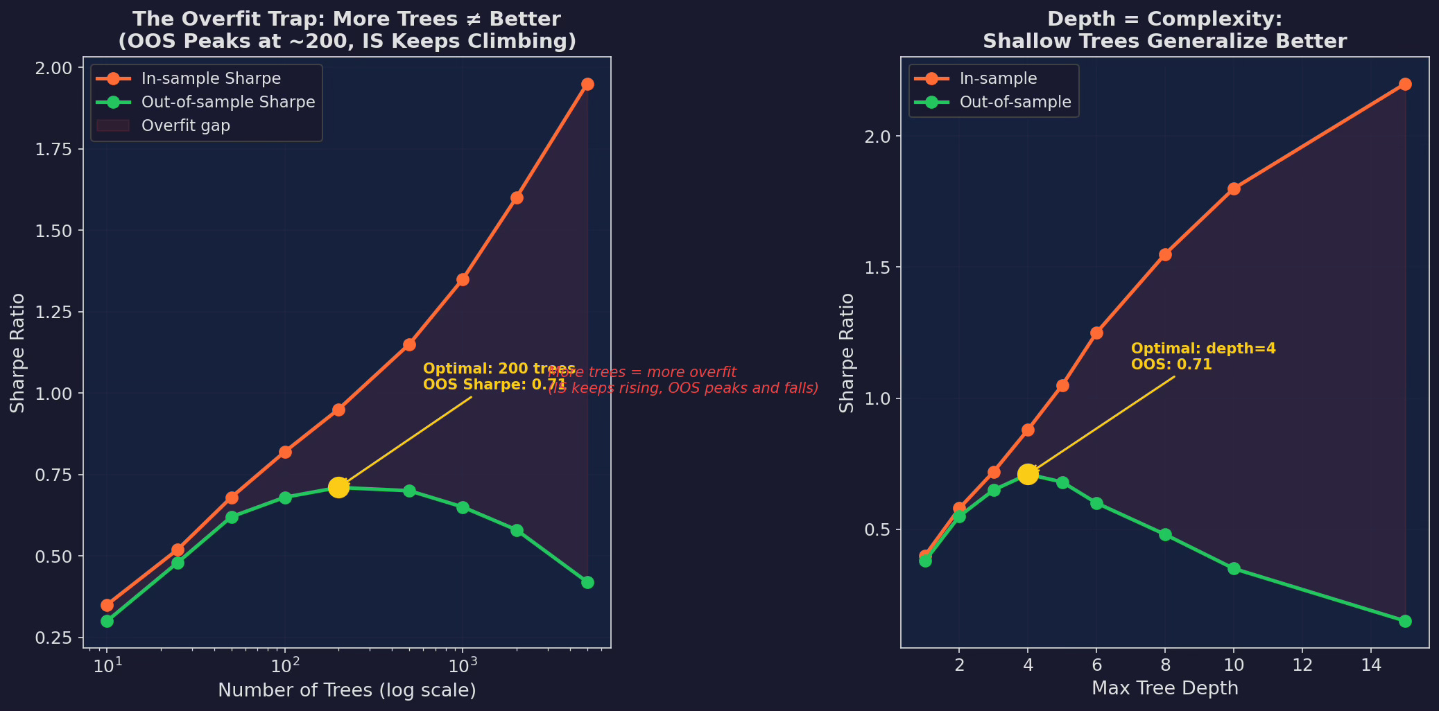
Left: number of trees vs. Sharpe. In-sample Sharpe climbs to 1.95 with 5,000 trees. Out-of-sample peaks at 200 trees (0.71) then declines to 0.42 with 5,000 trees. The widening gap is pure overfitting. Right: max tree depth shows the same pattern. Depth 4 is optimal OOS (0.71). Depth 15 gives an IS Sharpe of 2.20 and an OOS Sharpe of 0.15.

This is the central problem of ML for trading: the model that looks best in-sample is the worst out-of-sample.

A researcher who only reported the depth-15 IS Sharpe of 2.20 would have a “stunning” result. The actual OOS Sharpe of 0.15 tells you it’s garbage. The only honest approach is walk-forward validation with strict separation between parameter tuning and performance evaluation — which is what Part 97 (the overfitting minefield) will cover in depth.

For now, the practical takeaway: shallow trees, few estimators, heavy regularization. My final XGBoost configuration:

model = XGBRegressor(
    n_estimators=200,     # not 1,200 — OOS peaks here
    max_depth=4,          # shallow trees generalize better
    learning_rate=0.05,   # slow learning prevents overfitting
    subsample=0.7,        # row sampling (bagging)
    colsample_bytree=0.7, # column sampling (feature bagging)
    reg_alpha=1.0,        # L1 regularization
    reg_lambda=5.0,       # L2 regularization (heavy)
    min_child_weight=50,  # minimum samples per leaf
)

Every parameter choice limits the model’s ability to memorize the training data. The resulting model is weaker in-sample but more honest out-of-sample.

---

The Uncomfortable Question

The XGBoost improves V6’s Sharpe from 0.33 to 0.56. That’s meaningful. But the 50-line microstructure layer from Post 86 improved it from roughly 0.33 to roughly 0.50 (varying by simulation).

The marginal improvement of ML over hand-tuned rules is about +0.06 Sharpe. For that, you get:

Additional complexity:
  - Model training pipeline (data prep, validation, tuning)
  - Feature maintenance (11 features, daily updates)
  - Periodic retraining (quarterly, per Part 95's IC decay)
  - Monitoring for model drift
  - SHAP analysis for each trade decision

versus:

50 lines of if-else that anyone can read, modify, and debug

Is +0.06 Sharpe worth that operational burden? Part 98 will give the definitive answer. But I’ll preview my current thinking: it depends on your scale. At $100K, the if-else rules win on simplicity. At $10M+, the ML layer starts to justify its overhead.

---

Up Next

Part 97: The Overfitting Minefield — Walk-forward validation, combinatorial purged cross-validation, the deflated Sharpe ratio, and a rigorous framework for answering “is this result real or noise?”

---

Remember: Alpha is never guaranteed. And the backtest is a liar until proven otherwise.

These posts are about methodology, not recommendations. If you find errors in my math, let me know — I’ve built an entire series around discovering my own mistakes, so one more won’t hurt.

The material presented in Math & Markets is for informational purposes only. It does not constitute investment or financial advice.

---