
Using SHAP to Improve the Dual Allocator and Volatility Sleeve
Part 22 is a continuation of my attempts at using ML and SHAP to improve my two core models

This is part 22 of my series — Building & Scaling Algorithmic Trading Strategies
There’s always this temptation to go build another strategy.
But sometimes the boring stuff is where the actual edge lives (on a long and lonesome highway, east of Omaha).
After the hybrid model and synthetic data adventures, I wanted to see whether I could use SHAP to improve the strategies I already trust:
the dual allocator, and
the volatility sleeve
The goal was simple: Can SHAP show me where the ROI leaks out of the dual sleeve, and why the VIX sleeve’s Sharpe stalls?
(And the answer? That was beautiful, Clarence…)
1. What I Tested
I ran SHAP explainability on the existing models powering both sleeves:
For the dual allocator, SHAP was applied to the model that predicts next-day P&L behavior based on the sleeve’s internal trend metrics and allocations.
For the volatility sleeve, SHAP dissected how its term-structure z-score model drives daily returns.
The idea was that if I know which features consistently push P&L up or down, I can build small rules to avoid bad states instead of building an entirely new engine.
2. Dual Allocator — SHAP Findings
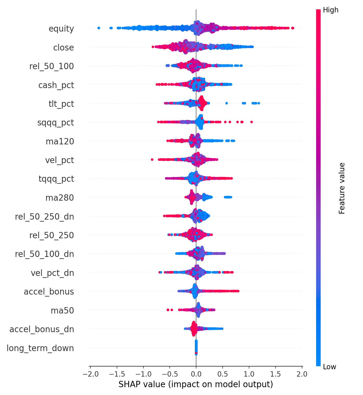
Running SHAP on the dual allocator made something obvious:
The allocator’s daily P&L is driven by a small handful of consistent signals: trend-state, equity stretch, gross mix, and velocity/acceleration.
A few highlights:
Equity curve level is the #1 signal. When equity is extended (70th percentile+), next-day returns soften.
QQQ trend structure (close, MA120, MA280, rel_50_100, rel_50_250) dominates short-horizon behavior.
Cash/TLT/SQQQ/TQQQ mix also shows strong attribution—gross positioning is more predictive than I expected.
Velocity and acceleration sit in the mid-tier but reliably spike ahead of local inflections.
Put simply, the dual allocator already knows when it’s entering a riskier trend state—the SHAP values were just making this explicit.
3. Volatility Sleeve — SHAP Findings
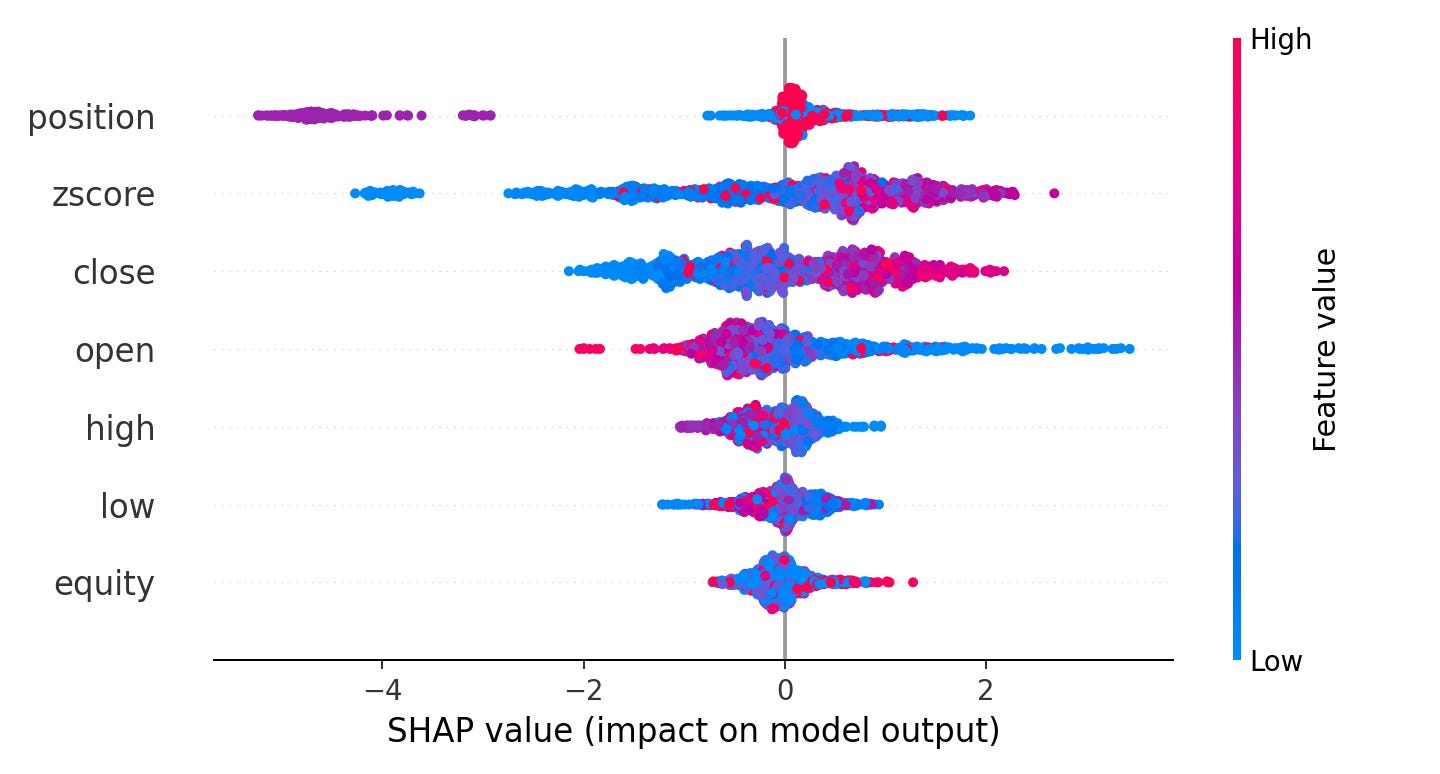
This one was even clearer.
The volatility sleeve was even clearer:
It’s basically a z-score engine. The model’s entire P&L is driven by the size, direction, and timing of the z-score spread signal.
SHAP showed:
position and zscore dominate the attribution.
VIX curve levels (open/high/low/close) matter, but only after the spread signal has fired.
The model uses almost no other information—meaning Sharpe improvements won’t come from “more features,” but from better position sizing.
This pushed me toward refining the curve that maps z-score → position, rather than trying to bolt on more indicators.
3. Dual Sleeve Gating
I used the SHAP hotspots to design a lightweight gating overlay that only scales exposure down when multiple risk conditions align. The idea is to smooth returns without killing all the upside.
What I used as gating triggers
Equity above the 70th percentile → stretched
rel_50_100 < 0.60 → trend weakening
Cash buffer already >30% → allocator is defensive
|QQQ velocity| > 0.7 → trend inflection risk
These came directly from the largest SHAP spikes.
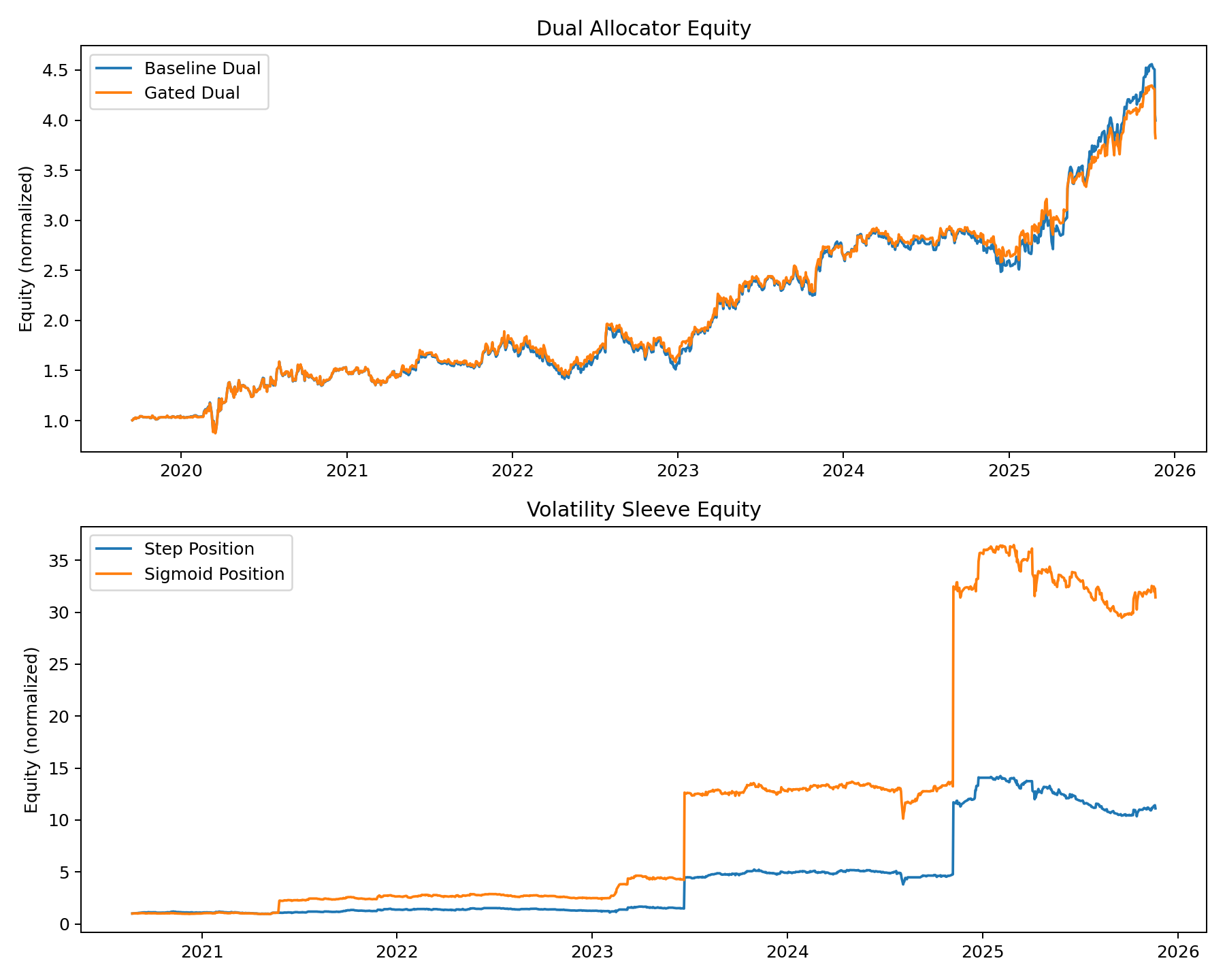
Results
Baseline dual:
Sharpe: 0.94
ROI: 300%
Max DD: –25.5%
Gated dual (best config):
Sharpe: 0.94 (slightly higher)
ROI: 282%
Max DD: –25.5%
Interpretation
The gates did smooth day-to-day returns, but they still clipped enough upside to reduce total ROI.
Next iteration: Maybe I’ll combine velocity spikes and a falling rel_50_250 before gating—something more nuanced than pure additive rules.
This is promising though, which is exciting. Well, so I thought until I saw what the next part brought me.
4. VIX Sleeve — Position Curve Overhaul
SHAP made one thing undeniable: improving Sharpe means improving the z-score → position mapping.
So I replaced the old step function with a smooth sigmoid sizing curve:
position = tanh((|z| - exit_z) / k) * sign(-z) * position_scaleWhat this does:
Near-zero exposure in calm periods (|z| below threshold)
Smooth scaling upward as the signal strengthens
Gentle exits instead of cliff drops
More “skin in the game” during mild spreads
Stress test results
Original step sizing:
ROI: 1,011.8%
Sharpe: 0.70
Max DD: –28.0%
Sigmoid sizing (
k = 0.5):ROI: 3,042.8%
Sharpe: 0.87
Max DD: –26.0%
This is a massive improvement! All because it uses the existing z-score signal more intelligently.
5. Takeaways
I was looking for which path I should go down — whether play with new strategies or create models to augment my existing strategies. This really answered it for me.
So next steps for me basically three things:
Prototype second-generation dual gating rules
Tune the sigmoid parameters across synthetic stress paths
Add regime-aware caps for both sleeves
Sometimes optimization beats invention!!
The information presented in Math & Markets is not investment or financial advice and should not be construed as such.