The Volatility Series, Part 6: Building a Volatility Surface

Part 65 — Volatility Series 6 of 7 — From raw option prices to a smooth, arbitrage-free surface

This is part 65 of my series — Building & Scaling Algorithmic Trading Strategies

---

In Part 63, we dove deep into the higher-order Greeks. Now we step back and ask a foundational question: where do those implied volatilities actually come from?

Well, we construct them from market prices. And that construction process — building a volatility surface — is both an art and a science.

This post covers:

1. Extracting IV from raw option prices

2. Choosing the right moneyness metric

3. Interpolation methods (spline, RBF, parametric)

4. The SABR and SVI models

5. Arbitrage-free constraints

6. Building the surface in Python

So let’s go build something!

---

1. From Prices to Implied Volatility

Every quoted option price has an implied volatility hiding inside it. The extraction is straightforward but computationally non-trivial.

The Inversion Problem

Given a market price $C_{mkt}$, we need to find σ such that:

Black-Scholes(S, K, T, r, σ) = C_mkt

There’s no closed-form solution. We use numerical methods:

from scipy.optimize import brentq
from scipy.stats import norm
import numpy as np

def black_scholes_call(S, K, T, r, sigma):
    if T <= 0 or sigma <= 0:
        return max(S - K, 0)
    d1 = (np.log(S / K) + (r + sigma**2 / 2) * T) / (sigma * np.sqrt(T))
    d2 = d1 - sigma * np.sqrt(T)
    return S * norm.cdf(d1) - K * np.exp(-r * T) * norm.cdf(d2)

def implied_vol(price, S, K, T, r):
    """Extract IV using Brent's method"""
    def objective(sigma):
        return black_scholes_call(S, K, T, r, sigma) - price
    
    try:
        return brentq(objective, 0.001, 5.0)
    except ValueError:
        return np.nan  # No solution (arbitrage or bad data)

The brentq method is reliable and fast — typically converges in 5-10 iterations.

Handling Edge Cases

Real market data is messy:

• Stale quotes: The bid/ask might not reflect current conditions

• Wide spreads: Use mid-price, but it might be off

• Deep OTM/ITM: Very small prices → large IV errors

• Near expiry: Small time value → numerical instability

I typically filter for:

• Bid > 0 (actually quoted)

• Spread < 50% of mid (reasonable liquidity)

• 10 < DTE < 365 (avoid extreme expirations)

• 0.80 < K/S < 1.20 (reasonable moneyness)

---

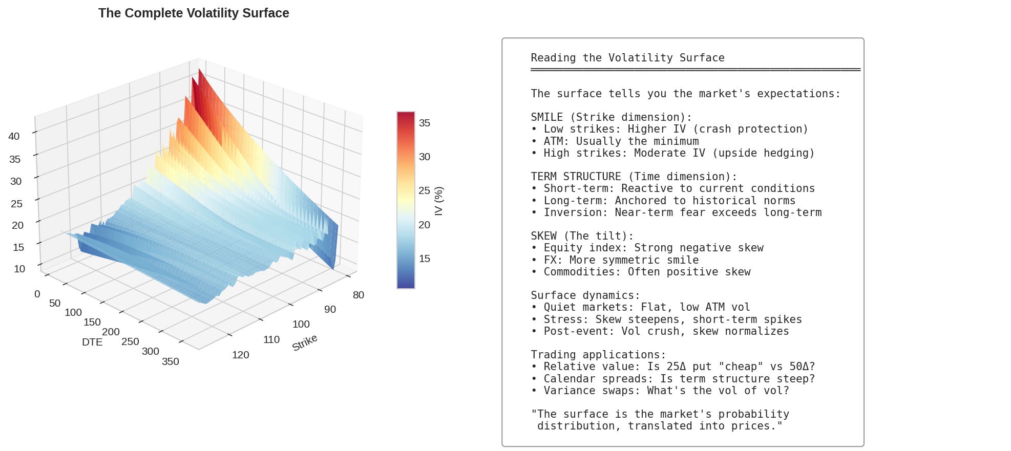
2. What the Raw Data Looks Like

Once you extract IVs for all available strikes and expirations, you get something like this:

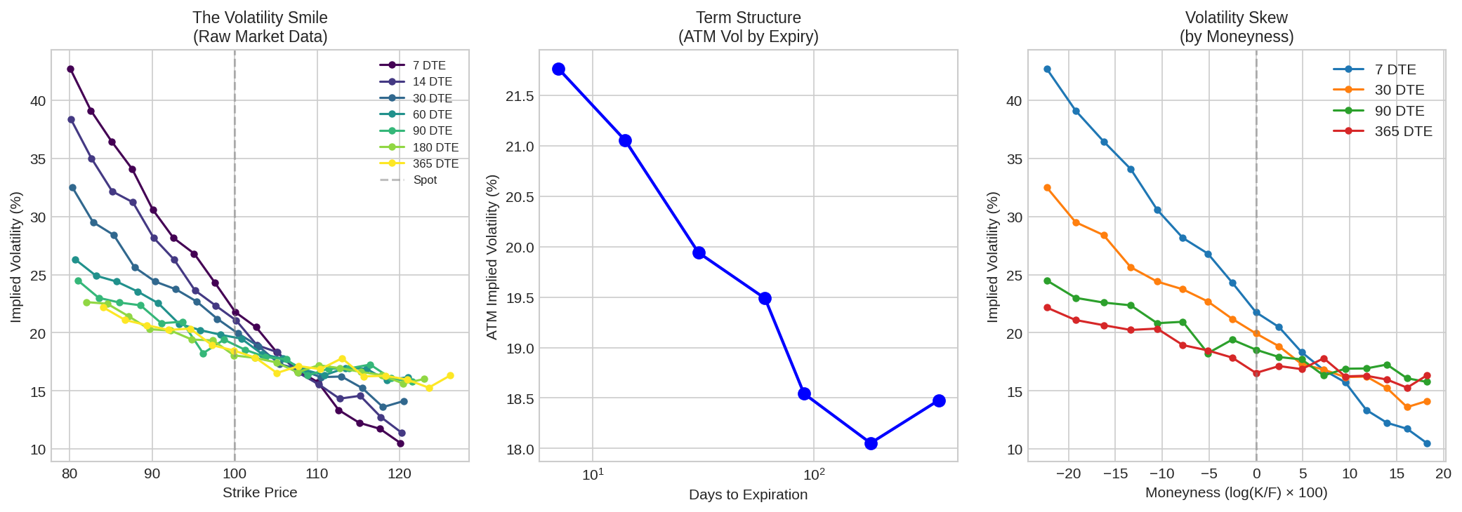
3 key features jump out:

The Smile: IV is higher for OTM options (both puts and calls) than ATM. This reflects the market’s belief in fat tails — extreme moves happen more often than Black-Scholes predicts.

The Skew: For equity indices, OTM puts have higher IV than OTM calls. This “skew” reflects crash fear — investors pay more for downside protection. The skew is steeper for short-dated options.

The Term Structure: Short-dated options often have higher IV than long-dated (especially in stressed markets). This reflects near-term uncertainty.

---

3. Choosing a Moneyness Metric

Before interpolating, you need to decide how to parameterize the strike dimension. Options include:

Strike (K): Simple, but not scale-invariant. A $100 option on a $100 stock is ATM; on a $200 stock, it’s deep OTM.

Moneyness (K/S or K/F): Scale-invariant, but doesn’t account for vol or time.

Log-moneyness: k = ln(K/F), where F is the forward price. This is the most common choice.

Delta: Parameterize by option delta (e.g., “25-delta put”). This is natural for FX markets and aligns with how traders think.

Standardized moneyness: m = ln(K/F) / (σ√T). This accounts for vol and time, making different expirations comparable.

For most equity work, log-moneyness is the standard choice:

k = ln(K/F)

Where:
  F = S × e^(r-q)T  (forward price)
  k < 0 → OTM put / ITM call
  k = 0 → ATM
  k > 0 → OTM call / ITM put

---

4. Building the Surface

With IVs extracted and moneyness defined, we need to interpolate between the observed points to create a continuous surface.

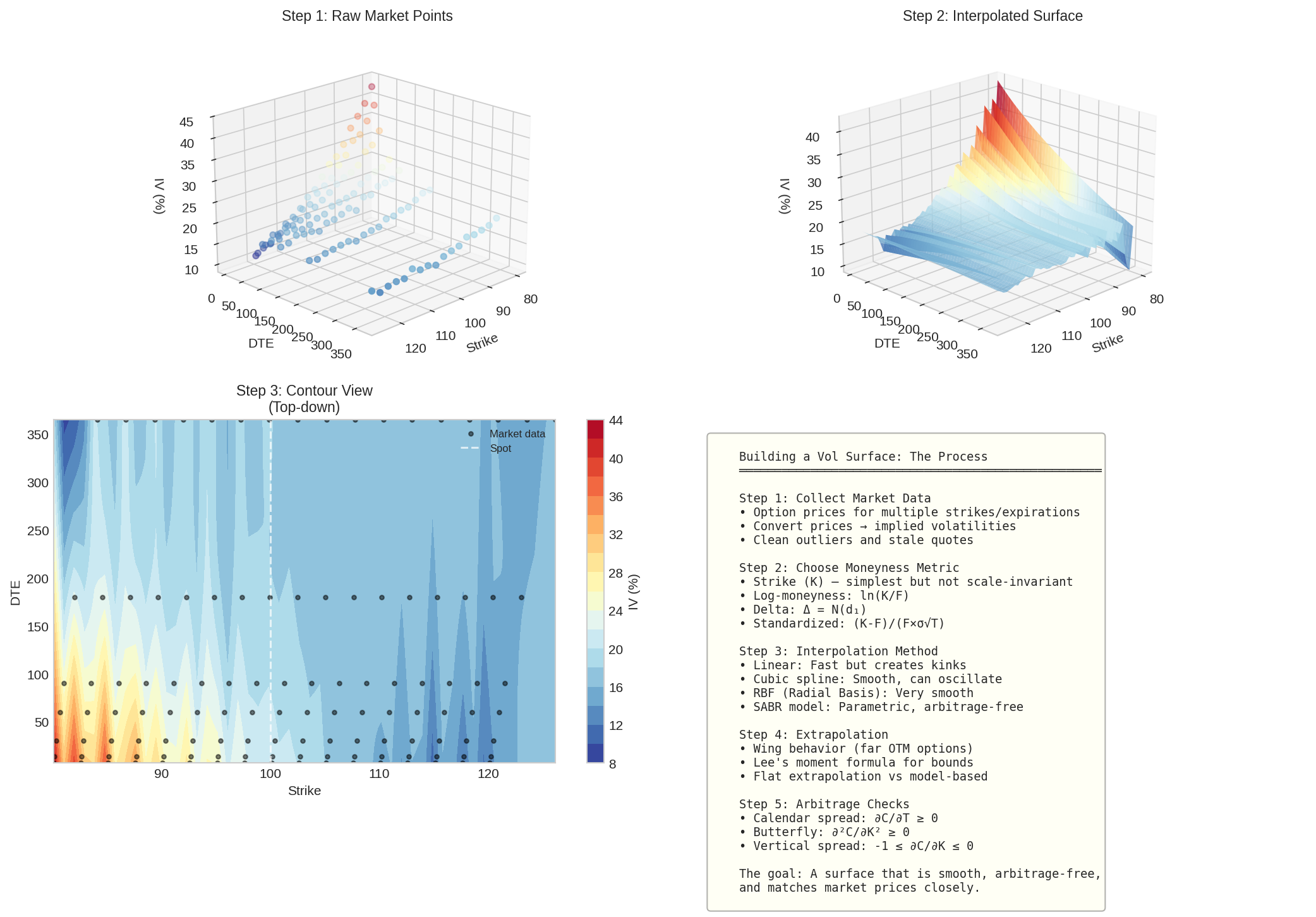
Method 1: Linear Interpolation

Simplest approach: connect the dots with straight lines.

Pros: Fast, no overshoot Cons: Creates kinks (discontinuous derivatives), looks ugly, Greeks are discontinuous

Not recommended except for quick-and-dirty work.

Method 2: Cubic Spline

Fit cubic polynomials between points, ensuring smooth derivatives at knots.

from scipy.interpolate import CubicSpline

# For each expiration, fit a spline in the strike dimension
spline = CubicSpline(strikes, ivs, bc_type='natural')

Pros: Smooth, well-behaved derivatives Cons: Can oscillate (Runge’s phenomenon) at the wings, not guaranteed arbitrage-free

(For any of my fellow math nerds, this is the same Carl Runge known for his Runge-Kutta method that some of us engineers had to learn in numerical analysis…)

Method 3: Radial Basis Functions (RBF)

Use a weighted sum of radial kernels centered at each data point:

from scipy.interpolate import RBFInterpolator

points = np.column_stack([strikes, times_to_expiry])
rbf = RBFInterpolator(points, ivs, kernel='thin_plate_spline', smoothing=0.001)

# Evaluate anywhere on the surface
iv_interpolated = rbf(np.array([[strike, tte]]))

Pros: Handles irregular grids, very smooth, works in 2D naturally Cons: Computationally expensive for large datasets, extrapolation can be wild

Method 4: Parametric Models

Instead of pure interpolation, fit a parametric model. The two industry standards are SABR and SVI.

---

5. The SABR Model

SABR (Stochastic Alpha Beta Rho) is the industry standard for interpolating volatility smiles, especially in fixed income and FX.

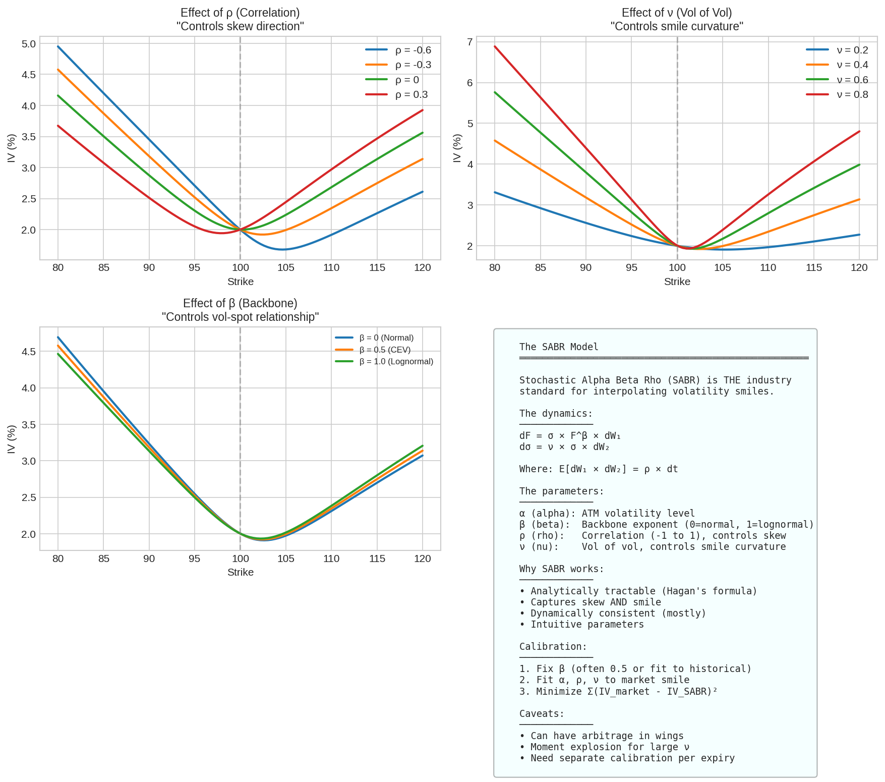
The Dynamics

dF = σ × F^β × dW₁     (forward price)
dσ = ν × σ × dW₂      (stochastic vol)

Where: E[dW₁ × dW₂] = ρ × dt

The forward price follows a CEV process (exponent β), and volatility itself is stochastic with vol-of-vol ν.

The Parameters

α (alpha): Controls the ATM volatility level. Higher α = higher ATM vol.

β (beta): The “backbone” parameter. β=0 is normal model, β=1 is lognormal. Most practitioners fix β=0.5 or estimate from historical data.

ρ (rho): Correlation between spot and vol. Negative ρ creates the skew (downward-sloping smile on the left).

ν (nu): Vol of vol. Higher ν = more smile curvature (fatter tails).

Hagan’s Approximation

The beauty of SABR is that there’s an analytical approximation for implied vol (Hagan et al., 2002):

σ_impl(K) ≈ α / (FK)^((1-β)/2) × z/x(z) × [1 + O(T)]

Where:
  z = ν/α × (FK)^((1-β)/2) × ln(F/K)
  x(z) = ln[(√(1-2ρz+z²) + z - ρ) / (1-ρ)]

The full formula is messier, but the key insight is that SABR gives you a closed-form smile from just 4 parameters.

Calibration

from scipy.optimize import minimize

def sabr_vol(F, K, T, alpha, beta, rho, nu):
    # Hagan's approximation (simplified ATM case shown)
    if abs(F - K) < 1e-10:
        return alpha / F**(1-beta) * (1 + T * (...))
    # ... full formula for non-ATM

def calibrate_sabr(F, K_market, iv_market, T, beta=0.5):
    def objective(params):
        alpha, rho, nu = params
        iv_model = [sabr_vol(F, K, T, alpha, beta, rho, nu) for K in K_market]
        return np.sum((np.array(iv_model) - np.array(iv_market))**2)
    
    result = minimize(objective, x0=[0.2, -0.3, 0.4], 
                      bounds=[(0.01, 2), (-0.99, 0.99), (0.01, 2)])
    return result.x

---

6. The SVI Model

SVI (Stochastic Volatility Inspired) parameterizes total variance rather than implied volatility:

w(k) = a + b × [ρ(k-m) + √((k-m)² + σ²)]

Where:
  k = ln(K/F) is log-moneyness
  w = σ² × T is total variance
  σ_impl = √(w/T)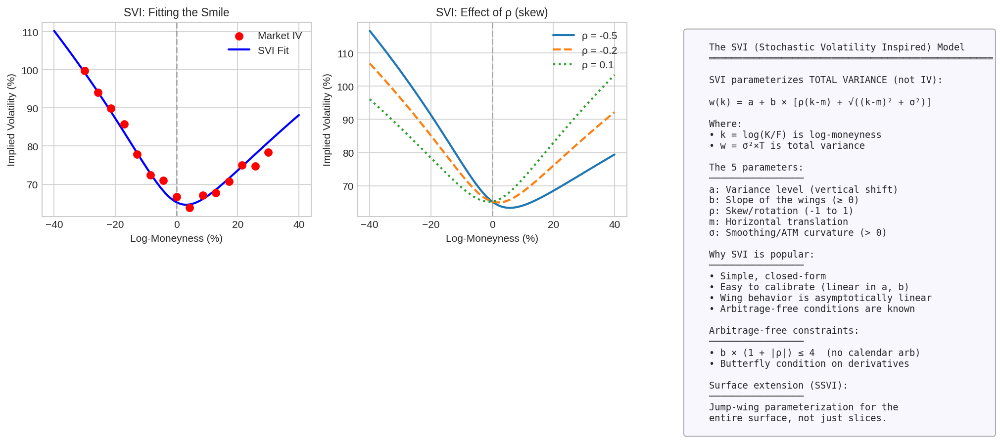

The Parameters

a: Variance level (vertical shift) b: Controls the slope of the wings (b ≥ 0) ρ: Skew/rotation parameter (-1 < ρ < 1) m: Horizontal translation σ: Controls ATM curvature (σ > 0)

Why SVI?

1. Simplicity: Just 5 parameters, closed-form

2. Wing behavior: Asymptotically linear wings (sensible extrapolation)

3. Arbitrage constraints: Well-understood conditions for no-arbitrage

4. Surface extension: SSVI extends this to the full surface

SVI Calibration

def svi_total_variance(k, a, b, rho, m, sigma):
    return a + b * (rho * (k - m) + np.sqrt((k - m)**2 + sigma**2))

def calibrate_svi(k_market, iv_market, T):
    def objective(params):
        a, b, rho, m, sigma = params
        w_model = [svi_total_variance(k, a, b, rho, m, sigma) for k in k_market]
        iv_model = np.sqrt(np.array(w_model) / T)
        return np.sum((iv_model - iv_market)**2)
    
    result = minimize(objective, x0=[0.02, 0.1, -0.2, 0, 0.1],
                      bounds=[(0, None), (0, None), (-0.99, 0.99), 
                              (-0.5, 0.5), (0.01, 0.5)])
    return result.x

---

7. Arbitrage Constraints

A valid volatility surface must be arbitrage-free. Three conditions must hold:

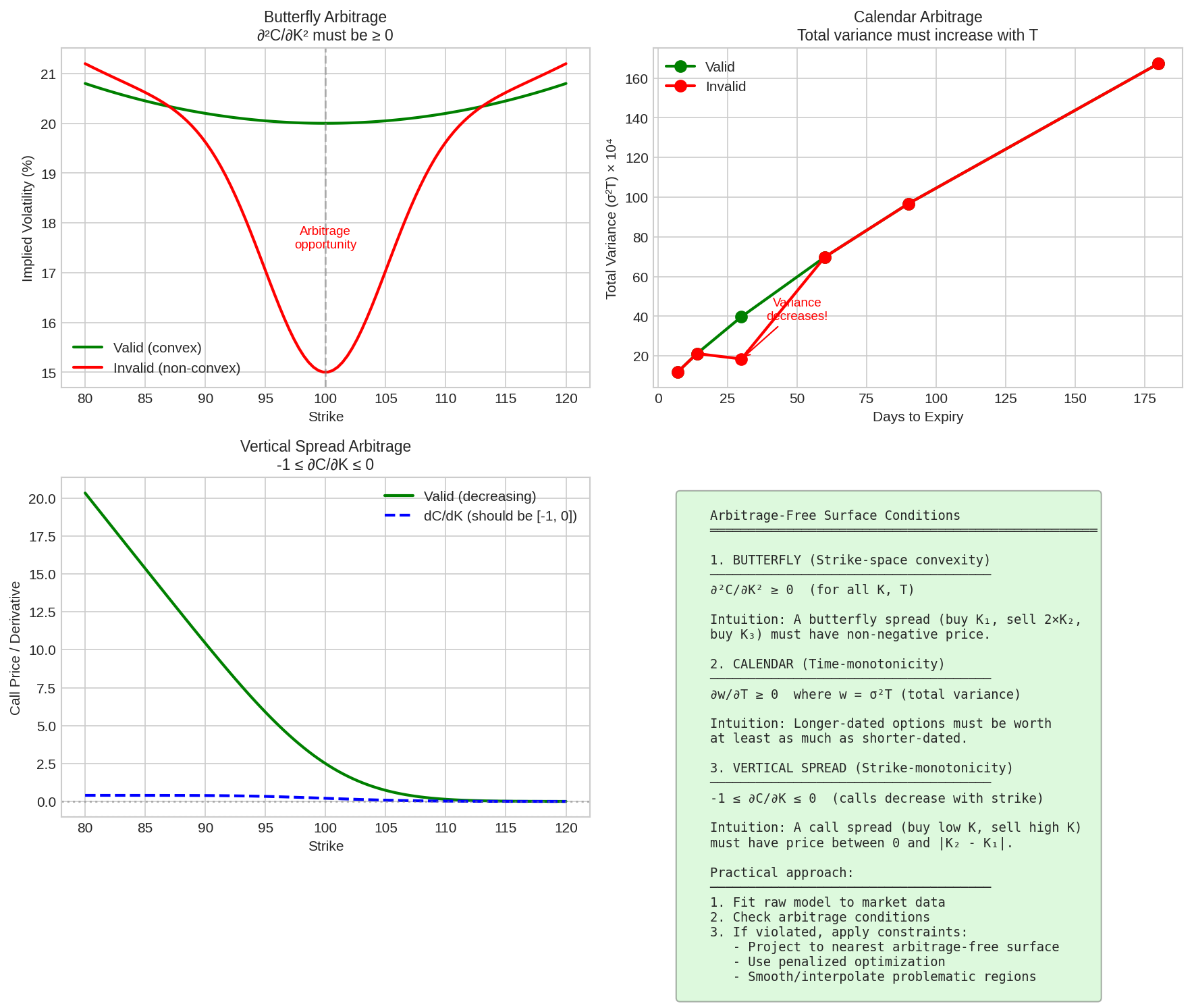
1. Butterfly Arbitrage (Strike Convexity)

∂²C/∂K² ≥ 0  for all K

This ensures a butterfly spread (buy K₁, sell 2×K₂, buy K₃) has non-negative price.

In IV terms: the implied volatility smile must be convex (or at least not concave).

Detection: Compute second derivative of call prices numerically. Any negative region = arbitrage.

2. Calendar Arbitrage (Time Monotonicity)

∂w/∂T ≥ 0  where w = σ²T (total variance)

Total variance must increase with time. Otherwise, you could buy the shorter-dated option, sell the longer-dated, and lock in risk-free profit.

Detection: Check that total variance is monotonically increasing along the time axis.

3. Vertical Spread Arbitrage (Strike Monotonicity)

-1 ≤ ∂C/∂K ≤ 0  for calls
 0 ≤ ∂P/∂K ≤ 1  for puts

Call prices must decrease with strike (but not faster than 1:1).

Detection: Compute ∂C/∂K numerically. Any values outside [-1, 0] = arbitrage.

Fixing Violations

If your interpolated surface violates arbitrage:

1. Smoothing: Increase the smoothing parameter in RBF or spline

2. Constrained optimization: Add arbitrage constraints to the calibration

3. Projection: Find the nearest arbitrage-free surface (complex but rigorous)

4. Use parametric models: SABR and SVI have known arbitrage-free parameter regions

---

8. The Complete Surface

Putting it all together:

Practical Workflow

1. Collect data: Pull option chains from your broker/data provider

2. Clean data: Remove stale quotes, filter by liquidity, use mid-prices

3. Extract IVs: Invert Black-Scholes for each option

4. Choose coordinates: Log-moneyness × time-to-expiry

5. Fit model: SABR per-expiry, or SVI/SSVI for full surface

6. Check arbitrage: Verify butterfly, calendar, vertical constraints

7. Store: Save parameters or interpolated grid for fast lookup

Code Snippet

def build_vol_surface(option_chain, S, r):
    """
    Build a complete volatility surface from raw option data.
    
    option_chain: DataFrame with columns [strike, expiry, bid, ask, type]
    S: current spot price
    r: risk-free rate
    
    Returns: callable function surface(K, T) → IV
    """
    # Step 1: Clean and filter
    df = option_chain.copy()
    df['mid'] = (df['bid'] + df['ask']) / 2
    df = df[df['bid'] > 0]  # Actually quoted
    df = df[(df['ask'] - df['bid']) / df['mid'] < 0.5]  # Reasonable spread
    
    # Step 2: Extract IVs
    df['T'] = (df['expiry'] - pd.Timestamp.now()).dt.days / 365
    df = df[df['T'] > 0.02]  # At least 1 week out
    
    df['iv'] = df.apply(lambda row: implied_vol(
        row['mid'], S, row['strike'], row['T'], r
    ), axis=1)
    
    df = df.dropna(subset=['iv'])
    
    # Step 3: Build interpolator
    points = df[['strike', 'T']].values
    ivs = df['iv'].values
    
    rbf = RBFInterpolator(points, ivs, kernel='thin_plate_spline', smoothing=0.001)
    
    # Step 4: Return callable
    def surface(K, T):
        return float(rbf(np.array([[K, T]])))
    
    return surface

---

9. Applications

Once you have a vol surface, you can:

1. Price exotic options: Use the local volatility derived from the surface

2. Calculate Greeks: Take numerical derivatives of the surface

3. Identify relative value: Is the 25-delta put “cheap” relative to the surface?

4. Backtest strategies: What would historical vol surfaces have looked like?

5. Manage Risk: Stress test your portfolio under surface shifts

---

10. Formula Reference

Implied Vol Extraction
──────────────────────
Solve: BS(S, K, T, r, σ) = C_mkt
Method: Brent's method on [0.001, 5.0]


Log-Moneyness
─────────────
k = ln(K/F)
F = S × e^(r-q)T


SVI Total Variance
──────────────────
w(k) = a + b[ρ(k-m) + √((k-m)² + σ²)]


SABR Implied Vol (ATM)
──────────────────────
σ_ATM ≈ α/F^(1-β) × [1 + T × correction_terms]


Arbitrage-Free Conditions
─────────────────────────
Butterfly: ∂²C/∂K² ≥ 0
Calendar:  ∂(σ²T)/∂T ≥ 0
Vertical:  -1 ≤ ∂C/∂K ≤ 0

---

11. Coming Up

• Part 66: Practical Vol Trading — possible approaches

---

Remember: Alpha is never guaranteed. And the backtest is a liar until proven otherwise.

Building vol surfaces requires careful attention to data quality. Garbage in, garbage out. Always validate your surface against market prices before using it for trading.

The material presented in Math & Markets is for informational purposes only. It does not constitute investment or financial advice.

---