
The Volatility Series, Part 1: Understanding the Fear Gauge
Part 60 — Volatility Series 1 of 7 — What volatility actually is, why it clusters, and how the VIX works

This is part 60 of my series — Building & Scaling Algorithmic Trading Strategies
This kicks off a new mini-series on volatility — in my view the single most important concept in options trading and a key input to many of the strategies I’ve built (including the Dual Allocator’s VIX regime gates and the 0DTE iron condors).
The goal is to build intuition from the math up. By the end of this series, you’ll understand:
What volatility actually measures (this post)
How the volatility surface works and why it has a “smile”
Trading strategies that exploit volatility mispricings
The Greeks — Vega, Gamma, Theta — and how they interact
1. What Is Volatility?
Volatility measures the dispersion of returns. Mathematically, it’s the standard deviation of log returns:
σ = √[ (1/n) × Σ(rₜ - r̄)² ]

Where:
  rₜ = ln(Pₜ / Pₜ₋₁)  — log return on day t
  r̄  = mean log return
  n  = number of observations
This gives daily volatility. To annualize (which is how volatility is typically quoted):
σ_annual = σ_daily × √252

Example:
  Daily vol = 1.2%
  Annual vol = 1.2% × √252 = 1.2% × 15.87 = 19.0%
The √252 factor assumes 252 trading days per year. This scaling works because variance (σ²) scales linearly with time, so volatility scales with the square root of time.
2. Realized vs Implied Volatility
Realized volatility (RV) is backward-looking — calculated from historical returns. It tells you what actually happened.
Implied volatility (IV) is forward-looking — extracted from option prices. It tells you what the market expects to happen.
The relationship:
Option Price = f(S, K, T, r, σ)

Given the market price, we solve for σ:
  IV = f⁻¹(Option Price, S, K, T, r)
IV is the volatility that, when plugged into Black-Scholes, produces the observed market price. It’s the market’s consensus forecast of future realized volatility.
The VIX premium is the typical gap between IV and subsequent RV:
VIX Premium = IV - Realized Vol (over next 30 days)
Historical average: ~3-4 percentage points
This premium exists because:
Investors pay up for downside protection (insurance premium)
Volatility has negative skew (big moves tend to be down)
Uncertainty about uncertainty (volatility of volatility)
3. Volatility Clustering
One of the most robust empirical facts about financial markets: volatility clusters. Large moves tend to follow large moves. Small moves tend to follow small moves.
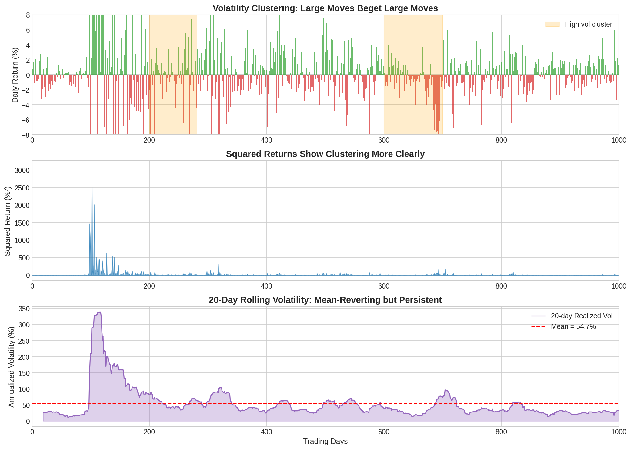
The chart shows this clearly:
Top panel: Daily returns. Notice how the big red/green bars cluster together (days 200-280, 600-700).
Middle panel: Squared returns (a variance proxy). The clustering is even more visible.
Bottom panel: Rolling 20-day realized volatility. It’s mean-reverting but persistent — high vol periods last for weeks or months.
Mathematically, this is captured by GARCH models:
σₜ² = ω + α × rₜ₋₁² + β × σₜ₋₁²

Where:
  ω = long-run variance weight
  α = reaction to recent returns (typically 0.05-0.15)
  β = persistence of volatility (typically 0.80-0.95)

α + β ≈ 0.95-0.99 (high persistence)
The GARCH(1,1) model says today’s variance depends on:
Yesterday’s squared return (the “shock”)
Yesterday’s variance (the “memory”)
With α + β close to 1, volatility shocks decay slowly. A VIX spike from 15 to 40 doesn’t snap back to 15 overnight—it decays over weeks.
This has direct trading implications:
After a volatility spike, expect elevated vol to persist
Mean reversion is real but slow
Selling vol after a spike is profitable on average but requires patience
4. How the VIX Works
The VIX is often called the “fear gauge,” but that’s an oversimplification. It’s actually a weighted average of implied volatilities across many SPX options.
The formula:
VIX² = (2/T) × Σ[ (ΔKᵢ/Kᵢ²) × e^(rT) × Q(Kᵢ) ] - (1/T) × (F/K₀ - 1)²

Where:
  T = time to expiry (30 days, interpolated)
  Kᵢ = strike price of option i
  ΔKᵢ = strike spacing
  Q(Kᵢ) = midpoint price of option at strike Kᵢ
  F = forward index level
  K₀ = first strike below forward
The key insight: VIX aggregates across all strikes, not just ATM. This means it captures the entire volatility surface—including the fat tails.
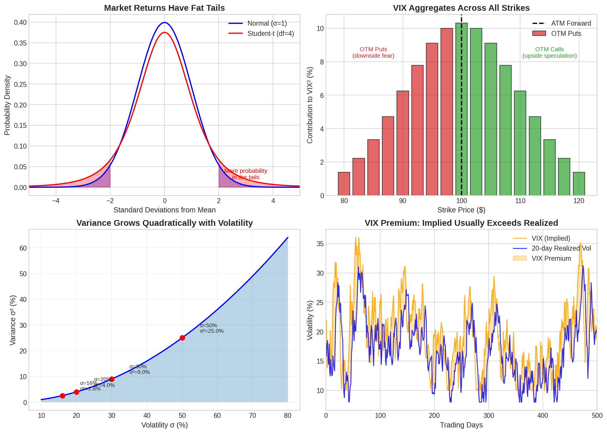
The panels show:
Fat tails: Market returns have heavier tails than a normal distribution (Student-t fits better). This is why OTM puts are expensive.
Strike contributions: VIX weights options by 1/K², so lower strikes (OTM puts) contribute more. This is why VIX spikes when people buy downside protection.
Variance vs volatility: Variance grows quadratically. A move from 16% to 32% vol means variance quadruples (2.56% → 10.24%). This non-linearity matters for variance swaps.
VIX premium: Implied typically exceeds realized by 3-4 points. This is the “insurance premium” embedded in options—and the source of premium-selling profits.
As an aside, I always have some amount of VIX ETFs in my portfolio so that I can actually monitor it as a tradeable asset — personally, I find that it gives me meaningful insight into how VIX is really performing at any time. I personally find a blend of VIXY and VIXM to be helpful canaries.
5. The Volatility Surface
Implied volatility isn’t constant across strikes and maturities. It varies systematically, forming a “surface.”
Key features:
The Smile: IV is higher for OTM options (both puts and calls) than ATM. This reflects fat tails — extreme moves happen more often than Black-Scholes predicts.
The Skew: IV is higher for OTM puts than OTM calls. This reflects negative skewness in returns — crashes are more common than melt-ups. The skew steepens during market stress.
Term Structure: Short-dated options often have higher IV than long-dated (especially in crisis). This reflects near-term uncertainty.
The surface parameters:
IV(K, T) = ATM(T) + Skew(T) × Moneyness + Smile(T) × Moneyness²

Where:
  Moneyness = ln(K/F)
  ATM(T) = at-the-money volatility at maturity T
  Skew(T) = slope of IV vs moneyness (typically negative)
  Smile(T) = curvature (typically positive)
Traders watch for:
Skew steepening: Fear increasing, puts getting bid
Skew flattening: Complacency, puts getting cheap
Term structure inversion: Near-term stress exceeding long-term expectations
6. Why This Matters for Trading
Volatility isn’t just an input to option pricing — it’s a tradeable asset class.
Long volatility (straddles, VIX calls): Profits when realized vol exceeds implied. Works in crashes and melt-ups.
Short volatility (iron condors, selling puts): Profits when realized vol is below implied. Collects the VIX premium.
Volatility arbitrage: Trading the spread between IV and expected RV, or between different parts of the surface.
The next post will cover volatility trading strategies in detail—how to structure trades that profit from volatility mispricings.
7. Key Formulas Reference
Annualized Volatility
─────────────────────
σ_annual = σ_daily × √252


Variance Scaling
────────────────
Var(T) = Var(1) × T
σ(T) = σ(1) × √T


GARCH(1,1)
──────────
σₜ² = ω + α × rₜ₋₁² + β × σₜ₋₁²


VIX Approximation (simple)
──────────────────────────
VIX ≈ √[ (2π/T) × Σ(ΔK/K²) × Put(K) ]  for K < F
    + √[ (2π/T) × Σ(ΔK/K²) × Call(K) ] for K > F


Black-Scholes Vega
──────────────────
Vega = S × √T × N'(d₁)
     = S × √T × (1/√2π) × e^(-d₁²/2)


Where:
  d₁ = [ln(S/K) + (r + σ²/2)T] / (σ√T)
8. Coming Up
Part 61: Volatility Trading Strategies — straddles, strangles, calendars, and when to use each
Part 62: The Greeks Deep Dive — Vega, Gamma, Theta, and their interactions
Part 63: Building a Volatility Surface — extracting and interpolating IV from market data
Part 64: Mean Reversion Strategies — trading the VIX premium systematically
Remember: Alpha is never guaranteed. And the backtest is a liar until proven otherwise.
These posts are about methodology, not recommendations. Some of the approaches discussed here involve complex instruments (e.g., options and derivatives) and not suitable for all investors. Many of my analyses probably contain errors — if you find them, please let me know.
While I may hold positions in some of the underlying assets discussed here, my posts are not an endorsement or a recommendation of those underlying assets.
The material presented in Math & Markets is for informational purposes only. It does not constitute investment or financial advice.