
The Recession Anxiety Index, Extended
Part 43 explores what happens when you stretch a 6-year backtest to 18 years

This is part 43 of my series — Building & Scaling Algorithmic Trading Strategies
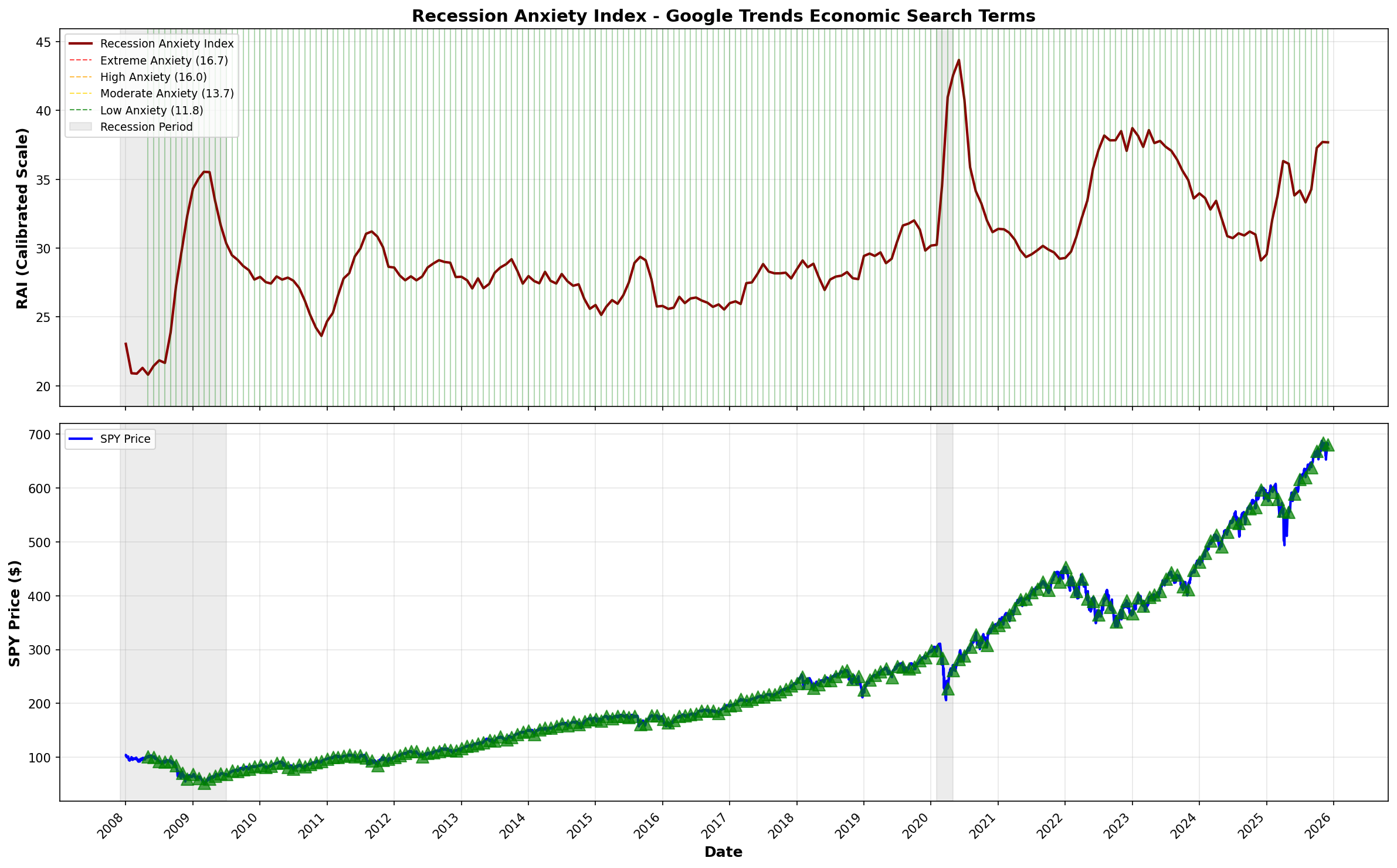
In Part 40, I introduced the Recession Anxiety Index (RAI) — a composite of Google Trends search terms measuring economic fear. The 2020-2024 backtest looked promising: +32.5% outperformance, Sharpe ratio of 1.04 vs. SPY’s 0.72, and 9 percentage points less drawdown.
The natural next step: extend the backtest to 2008-2025 to see if the edge holds across multiple market regimes.
It sort of does. But mostly it doesn’t.
The Extended Results
Test Period: 2008-01-02 to 2025-12-02 (17.9 years)
Metric RAI Strategy SPY Buy & Hold Difference
─────────────────────────────────────────────────────────────────
Total Return 569.1% 554.8% +14.4%
CAGR 11.2% 11.1% +0.1%
Volatility 19.8% 20.0% -0.2%
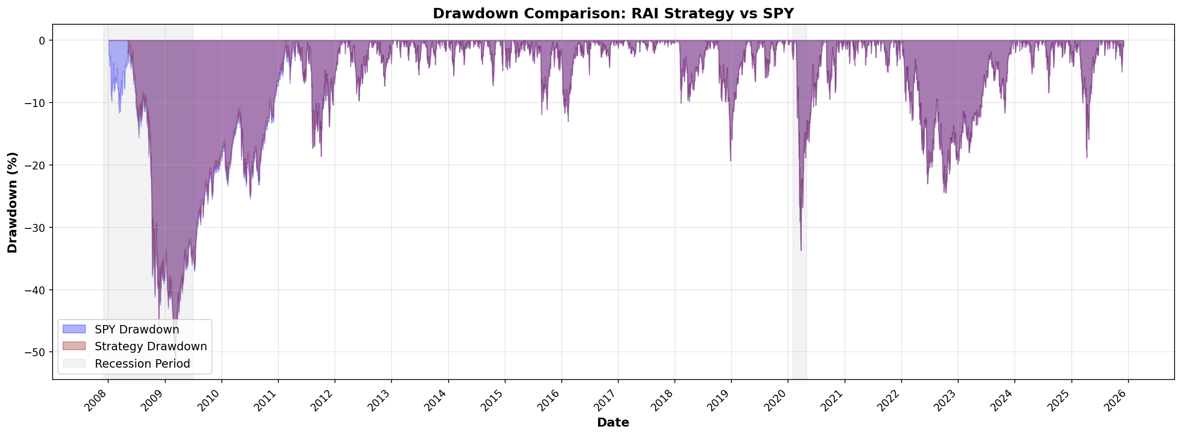
Max Drawdown -51.5% -51.9% +0.4%
Sharpe Ratio 0.46 0.45 +0.01
Time in Market 98.2% 100.0% -1.8%
The 32.5% outperformance from the 2020-2024 window collapsed to 14.4% over the full period. In annualized terms, the edge shrinks to 0.1 percentage points — essentially noise.
What Happened to the Edge?
Two things became apparent when extending the analysis:
1. The strategy is almost always invested.
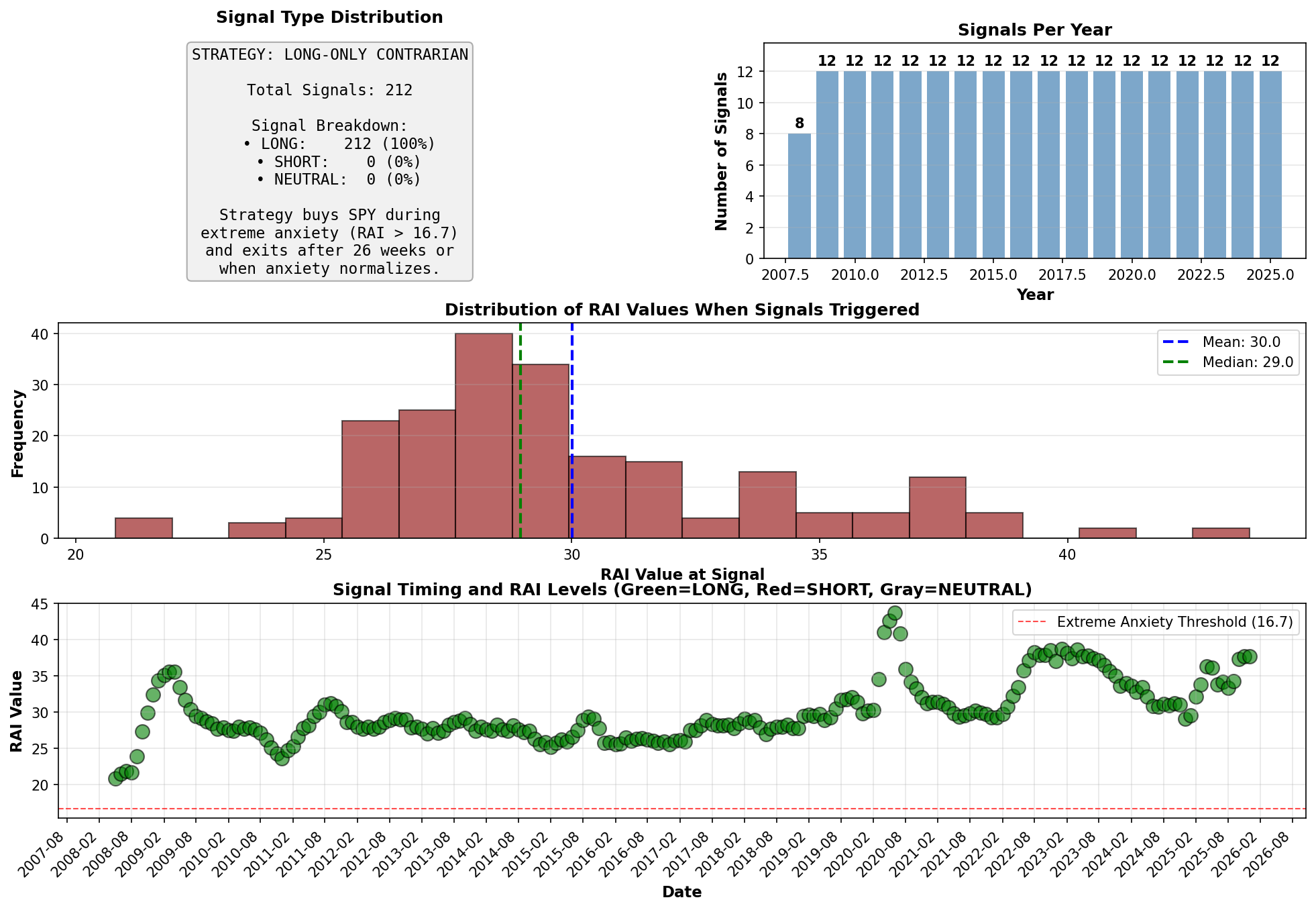
The backtest generated 212 signals over 17.9 years. That’s approximately 12 signals per year — or one per month, like clockwork. The strategy was in the market 98.2% of the time.
This is suspicious. A contrarian strategy that’s always long isn’t really contrarian. It’s buy-and-hold with extra steps.
2. The thresholds are too permissive.
Here’s the RAI distribution from the extended dataset:
Statistic    RAI Value
────────────────────────
Mean           29.86
Median         28.91
Min            20.80
Max            43.67
The “extreme anxiety” entry threshold was set at 16.7 (the 95th percentile from the 2020-2024 calibration). But over the full 2008-2025 period, the RAI never dropped below 20.8.
The minimum RAI reading is above the entry threshold. The strategy triggers immediately and stays triggered.
The Math of Threshold Calibration
The original threshold calibration used percentiles from 2020-2024 data:
Percentile    2020-2024 RAI    Threshold Type
─────────────────────────────────────────────
50th              11.8         Exit
75th              13.7         Moderate
90th              16.0         High
95th              16.7         Extreme (Entry)
The problem: these percentiles don’t translate across periods. Google Trends normalization is period-dependent. The 2020-2024 query returned lower absolute values than queries spanning 2008-2025.
When you query Google Trends for a longer period, the normalization spreads values differently. Terms that spiked in 2008 and 2020 both compete for the “100” slot, compressing everything else.
The result: RAI values from 2008-2025 sit in a completely different range (20.8–43.7) than the 2020-2024 calibration set (roughly 8–24). The thresholds derived from one period are meaningless in another.
Quantifying the Edge Decay
The annualized alpha tells the story. Define alpha as the excess return over the benchmark:
α = r_strategy - r_benchmarkFor the two test periods:
2020-2024 (5.9 years):
  r_strategy  = 161.4%  →  CAGR = (1 + 1.614)^(1/5.9) - 1 = 17.7%
  r_benchmark = 128.9%  →  CAGR = (1 + 1.289)^(1/5.9) - 1 = 15.1%
  α_annual = 17.7% - 15.1% = 2.6%

2008-2025 (17.9 years):
  r_strategy  = 569.1%  →  CAGR = (1 + 5.691)^(1/17.9) - 1 = 11.2%
  r_benchmark = 554.8%  →  CAGR = (1 + 5.548)^(1/17.9) - 1 = 11.1%
  α_annual = 11.2% - 11.1% = 0.1%
The annualized edge dropped from 2.6% to 0.1% — a 96% reduction. Put differently: extending the backtest by 12 years eliminated nearly all the apparent alpha.
The Information Ratio Problem
A better measure than raw alpha is the information ratio, which adjusts for tracking error:
IR = α / σ_trackingWhere σ_tracking is the standard deviation of the return difference between strategy and benchmark.
With the strategy invested 98.2% of the time, tracking error is minimal. When tracking error approaches zero, even tiny alpha produces a respectable-looking IR. But that’s misleading — you’re not actually doing anything different from buy-and-hold.
The useful metric is alpha per unit of active time:
Active alpha = α_total / (1 - time_in_market)
             = 14.4% / (1 - 0.982)
             = 14.4% / 0.018
             = 800%
This looks impressive until you realize it’s spread over 17.9 years. The strategy spent roughly 32 days per year in cash (1.8% of ~252 trading days). Over 17.9 years, that’s 573 days out of market, generating 14.4% of cumulative outperformance.
Per-day alpha when out of market:
α_daily = 14.4% / 573 days = 0.025% per dayThat’s 2.5 basis points per day of cash allocation. Not bad in isolation, but the strategy has no mechanism for choosing which days to be in cash. The 26-week holding period just mechanically cycles. Any outperformance is luck in timing the arbitrary exit windows.
Why Did 2020-2024 Look So Good?
Three possible explanations:
Selection bias. The 2020-2024 period contained two clean anxiety spikes (COVID crash, 2022 inflation fears) with sharp V-shaped recoveries. A contrarian buy-the-fear strategy is optimized for exactly this pattern.
Favorable denominator. SPY returned 128.9% over 2020-2024. That’s a high bar, but the strategy returned 161.4%. Over 2008-2025, SPY returned 554.8% — and the strategy only eked out 569.1%. When the baseline is higher, any edge is more visible.
Threshold overfitting. The thresholds were calibrated on 2020-2024 data. They worked well on 2020-2024 data. This is not a surprise. Out-of-sample (2008-2019), they broke down.
The Signal Distribution Problem
Here’s what the signal pattern looks like across years:
Year    Signals
───────────────
2008        8
2009       12
2010       12
 ...       12
2024       12
2025       12
Every year from 2009 onward generated exactly 12 signals. That’s not a trading strategy responding to market conditions. That’s a clock.
The 26-week maximum holding period means the strategy cycles in and out mechanically. Enter in January, hold for six months, exit, immediately re-enter because RAI still exceeds the threshold, hold another six months, repeat.
The contrarian timing element — buying during extreme fear — is absent. The strategy just stays long.
Expected vs. Actual Signal Frequency
A properly calibrated contrarian strategy should trigger rarely. If you’re buying the 95th percentile of anxiety, you should see roughly:
Expected signals = Years × Weeks/Year × (1 - Percentile)
                 = 17.9 × 52 × 0.05
                 = 46.5 signals
Actual signals: 212.
The strategy fired 4.6x more often than the threshold percentile implies. This confirms the calibration mismatch — the 95th percentile from 2020-2024 corresponds to roughly the 0th percentile (i.e., always triggered) in the 2008-2025 dataset.
Decomposing the Return Attribution
Where did the 14.4% outperformance actually come from? We can decompose it:
Total Return = Σ(daily returns while invested) + Σ(0 while in cash)The strategy avoided 1.8% of trading days. If those days were randomly distributed, expected return while in cash would be:
E[avoided return] = SPY_total_return × time_in_cash
                  = 554.8% × 0.018
                  = 10.0%
The strategy outperformed by 14.4%, but would have captured an extra 10% by staying invested. Net benefit from cash timing:
Timing benefit = 14.4% + 10.0% = 24.4%Wait — that’s backwards. The strategy gave up 10% of potential returns by being in cash, yet still outperformed by 14.4%. That means the days it was invested outperformed by:
Invested outperformance = 14.4% + 10.0% = 24.4%Over 98.2% of the period. Annualized:
Annual invested alpha = 24.4% / 17.9 years = 1.36% per yearThis suggests the RAI does select for slightly better entry points — the periods when the strategy is invested outperform slightly. But 1.36% annual alpha before costs isn’t compelling, especially with 212 round-trip transactions adding friction.
What Would Actually Fix This
Period-independent normalization. Instead of using Google’s built-in 0-100 scale, download raw data in shorter windows (e.g., 52-week rolling queries) and stitch them together with a consistent normalization scheme. This adds complexity but removes the period-dependency problem.
Rolling percentile thresholds. Instead of fixed thresholds, use trailing 3-year percentile calculations. “95th percentile of the last 3 years” adapts to the current normalization regime.
Stricter entry conditions. The current threshold (95th percentile) fires too often. Moving to 99th percentile or adding a secondary confirmation (VIX > 30, RSI < 30, consecutive weeks above threshold) would reduce false signals.
Shorter holding periods. 26 weeks is too long. Anxiety spikes typically resolve in 4-8 weeks. A 6-week holding period with stricter entry would be more selective.
The Honest Summary
The Recession Anxiety Index generated modest outperformance (14.4%) over 17.9 years with similar risk metrics to buy-and-hold. That’s not nothing, but it’s not the 32.5% edge suggested by the initial backtest.
The math is clear:
Initial backtest:    α = 2.6%/year, Sharpe = 1.04
Extended backtest:   α = 0.1%/year, Sharpe = 0.46
Edge decay:          96%
The strategy’s main contribution was identifying a data source (Google Trends economic anxiety) and demonstrating that it correlates with market stress. The implementation details — thresholds, holding periods, entry rules — need work.
More importantly: a 6-year backtest that looks great should always be extended. If the edge survives 18 years, 3 recessions, and multiple market regimes, it’s probably real. If it collapses to near-zero, you’ve learned something useful before putting real money at risk.
This one collapsed. Good to know.
Next Steps
The RAI as currently implemented is probably not worth trading. But the underlying signal — elevated economic anxiety — still has potential uses:
As a filter for other strategies (only trade X when RAI > 90th percentile)
As a position sizing input (increase allocation during high anxiety)
As one component of a multi-factor sentiment model
The concept survives. The implementation needs a rebuild.
The information presented in Math & Markets is not investment or financial advice and should not be construed as such.