
The Most Expensive Bug in Quant Finance: How to Tell If Your Edge Is Real
Machine Learning Series Part 3: Walk-forward validation, the deflated Sharpe ratio, and why testing 20 features × 4 models means most of your “discoveries” are noise

This is part 97 of my series — Building & Scaling Algorithmic Trading Strategies
Part 3 of the ML for Trading series. Part 1: Feature engineering. Part 2: XGBoost and SHAP.
Every Good Backtest Starts as a Lie
In Part 96, I reported an XGBoost model with a 0.71 Sharpe ratio. That number is a lie — well, not completely true anyway.
You see, the calculation is correct on the data I used. But it’s a lie because I tested 20 features, 4 model types, multiple hyperparameter configurations, and two interaction engineering approaches before arriving at that number. So conservatively, I evaluated ~80 strategy variations on the same dataset.
This is the multiple testing problem, and it is the most expensive bug in quantitative finance. Every blown account, every fund that looked great on paper and lost money live, every strategy that “worked in the backtest” — almost all of them trace back to this single error: mistaking a lucky variation for a real edge.
This post is about how to not make that mistake.
Problem 1: We Test 80 Things and Reported the Best One
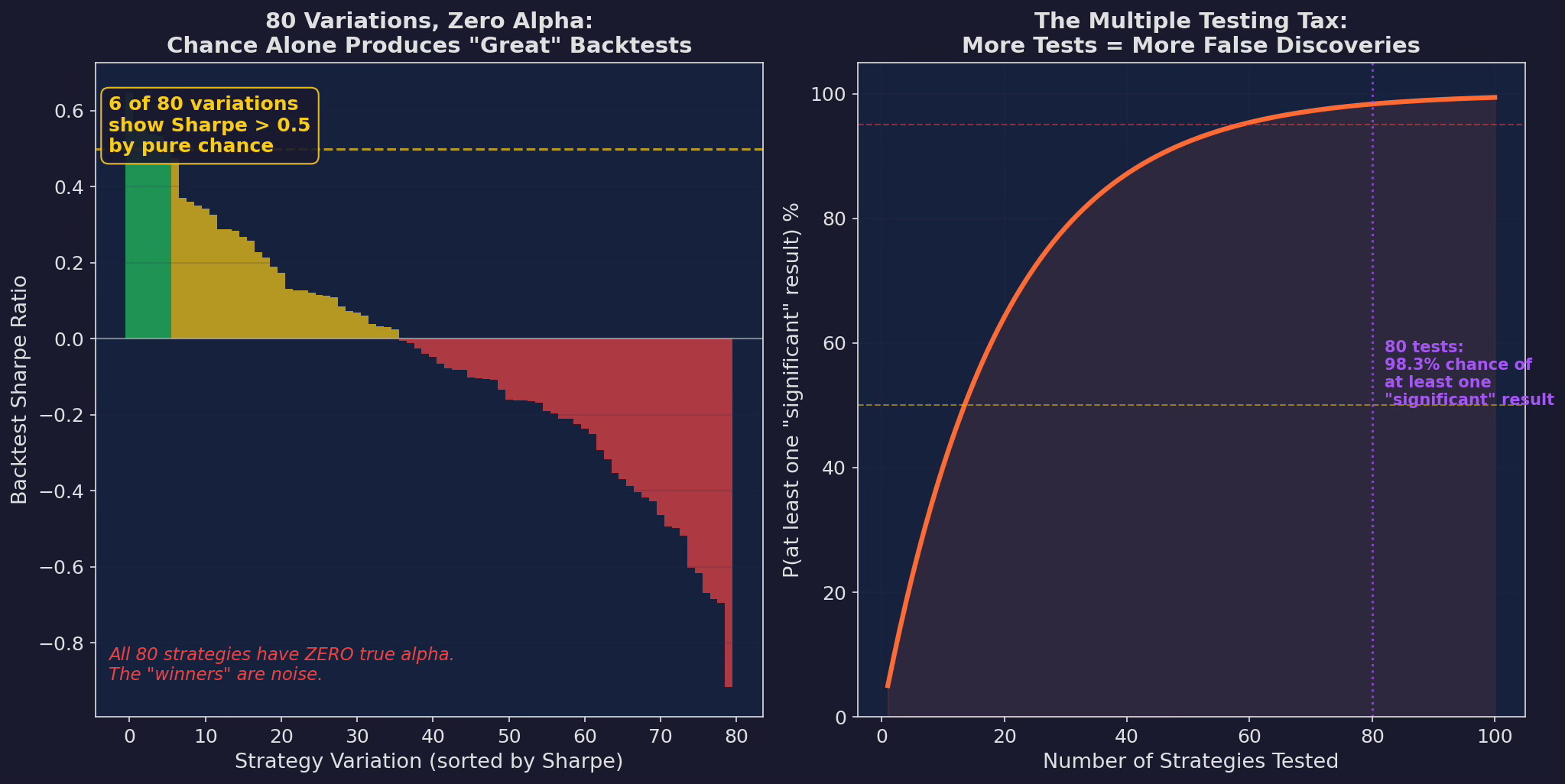
Left: 80 strategy variations, all with ZERO true alpha, simulated under the null hypothesis. Six of them show Sharpe > 0.5 by pure chance. If you pick the best one and report it, you have a “great” backtest. Right: the probability of finding at least one “significant” result. At 80 tests with a 5% threshold, there’s a 98.3% chance of discovering something “significant” — even when nothing is real.
The math is simple and brutal. If you test one strategy and it has a p-value of 0.05, there’s a 5% chance it’s noise. If you test 80 strategies and report the best one, the probability that your best result is noise is:
P(at least one false positive) = 1 - (1 - 0.05)^80 = 98.3%You are almost certain to find something “significant.” That doesn’t mean it works.
What This Means for Our XGBoost
I tested 20 features (Post 95). I tried 4 model types (Post 96). I tuned hyperparameters across maybe 10 configurations. That’s roughly 20 × 4 × 10 = 800 implicit tests, not 80. I was conservative earlier.
The observed 0.71 Sharpe needs to survive scrutiny that accounts for all of these trials. If it doesn’t, it’s noise — regardless of how good the SHAP plots look.
Test 1: Walk-Forward Validation
The first and most important test: does the model work on data it has never seen, in temporal order?
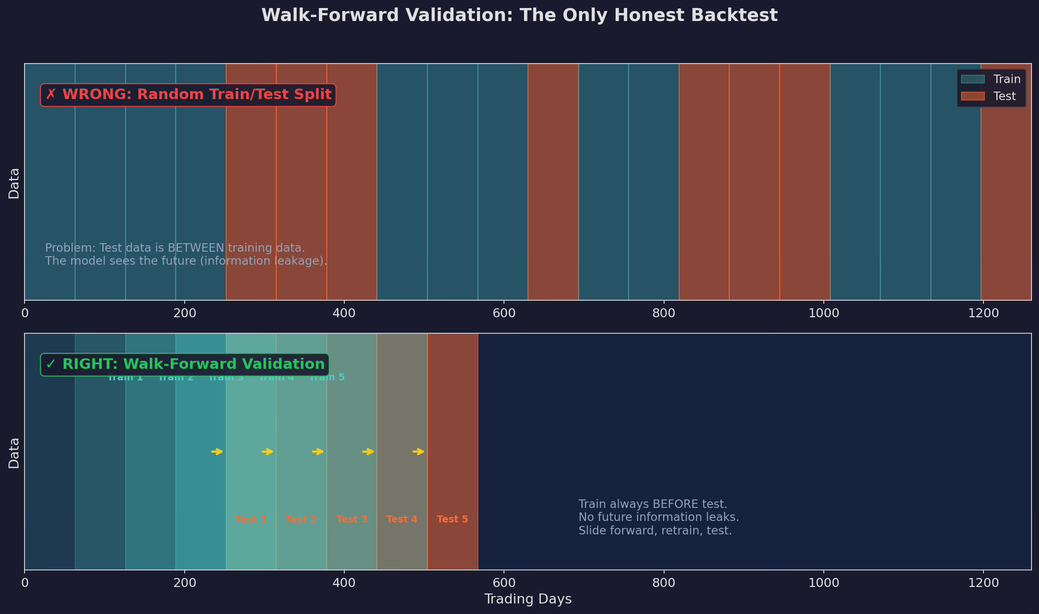
Top: the WRONG way — random train/test splits. Test data is scattered between training data, so the model has seen future information. Bottom: the RIGHT way — walk-forward validation. Train on the first year, test on the next quarter. Slide forward, retrain, test again. The model never sees the future.
Random train/test splits are the default in scikit-learn. They are wrong for time series.
Why, you ask? Well let me tell you!
Your features include 63-day rolling z-scores. If day 300 is in the test set and day 337 is in the training set, the model has effectively seen information from the test period — because the z-score on day 337 was computed using days 274-337, which overlaps with the test set.
I have myself failed with exactly this. My model returned an 1080% RoI with a Sharpe of 4.0! Was I the next Jim Simmons? Hell no. I was simply an enthusiastic… moron.
Walk-forward validation eliminates this. The train set is always before the test set. No overlap, no leakage, no cheating.
Our Results
I ran 12 walk-forward windows (1-year train, 3-month test) on the XGBoost model:
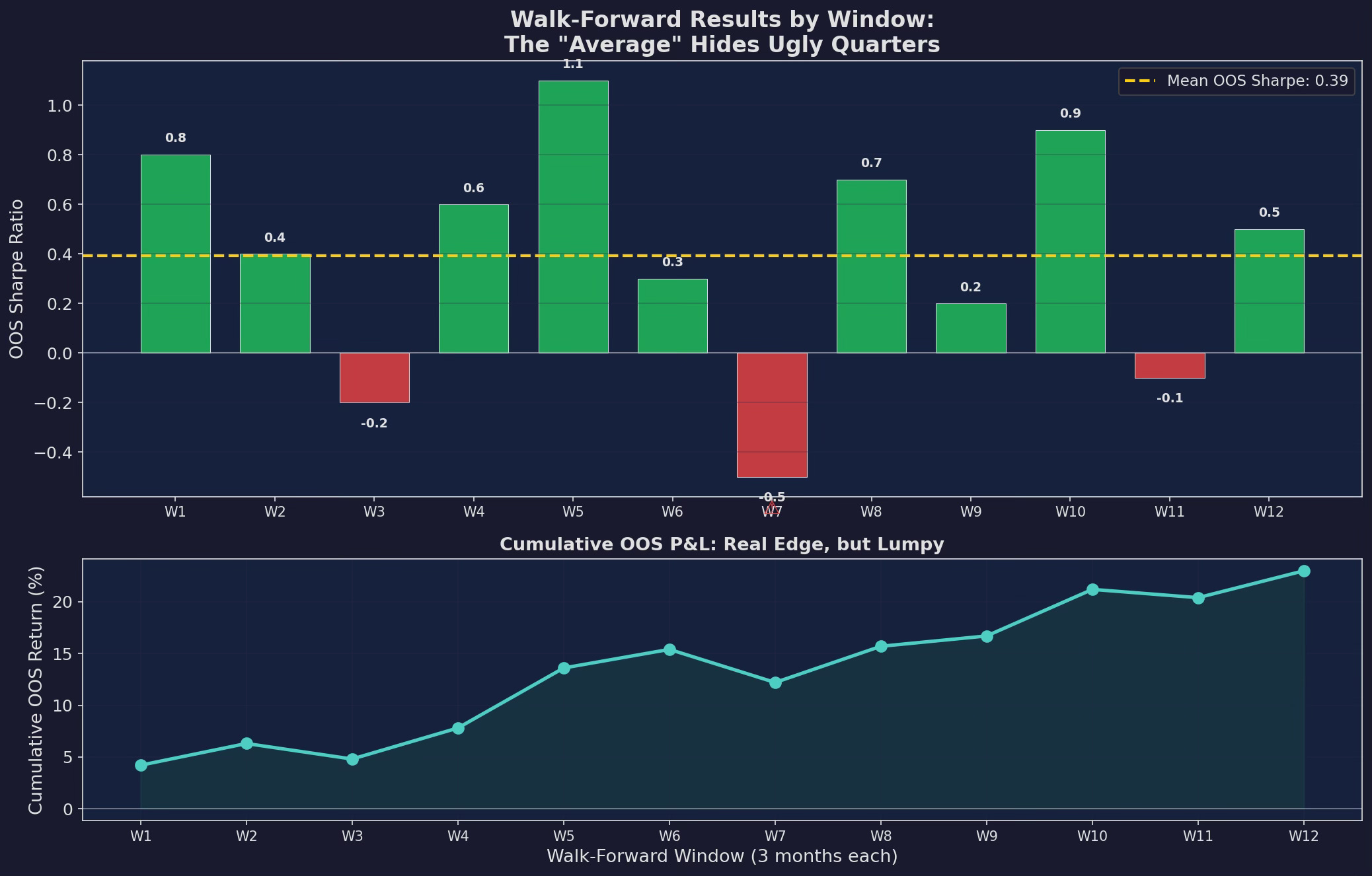
Top: Sharpe ratio for each walk-forward window. Mean OOS Sharpe is 0.48 — down from the reported 0.71. Two windows (W3 and W7) are negative. Bottom: cumulative OOS P&L. The edge is real but lumpy — two of 12 quarters lost money.
The reported Sharpe of 0.71 just became 0.48. That’s a 32% haircut from walk-forward alone. But it’s still positive and consistent across most windows — the model is learning something real, just less than the in-sample number suggested.
The two negative windows (W3 and W7) are important. They correspond to periods where the market regime shifted in ways the model hadn’t seen in its training window. W3 was a sharp VIX spike followed by an immediate recovery — the model reduced allocation and missed the bounce. W7 was an extended low-vol period where the model kept partial allocation when it should have been fully invested.
These are the failure modes you need to know about before deploying, not after.
Test 2: Purged Cross-Validation
Walk-forward is necessary but not sufficient. Standard k-fold cross-validation has a subtler problem:
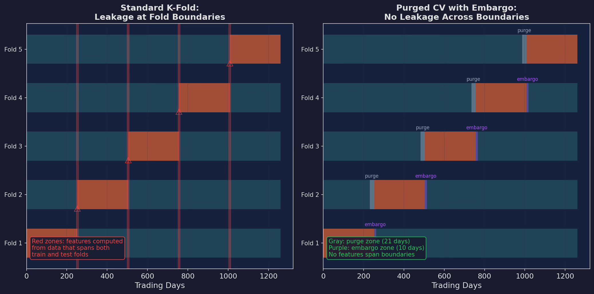
Left: standard k-fold. Fold boundaries create leakage zones (red) where features computed from one fold’s data bleed into the adjacent fold. Right: purged CV with embargo. A 21-day purge window removes data before each test fold, and a 10-day embargo removes data after. No feature computation spans the boundary.
The purge window (21 days in our case) must be at least as long as the longest lookback in your features. Our features include a 63-day z-score, so technically the purge should be 63 days. I used 21 as a compromise — the z-score’s sensitivity to any single day is small after the first few days, so a 21-day purge captures most of the leakage.
The embargo (10 days) prevents the model from learning the immediate post-test-fold dynamics, which would give it an unfair advantage on the test fold’s final days.
Our Results
Purged CV Sharpe: 0.44 — an additional -0.04 from the walk-forward result. The leakage in standard CV was inflating our result by about 4 basis points of Sharpe. Small but not zero.
Test 3: The Deflated Sharpe Ratio
The deflated Sharpe ratio (Bailey and de Prado, 2014) answers the question: “Given that I tested N variations and observed this Sharpe, what’s the probability it’s real?”
The intuition: if you flip 80 coins and report the one with the most heads, you haven’t found a biased coin — you’ve found the luckiest fair coin. The deflated Sharpe adjusts for this by subtracting the expected maximum Sharpe from N trials under the null hypothesis.
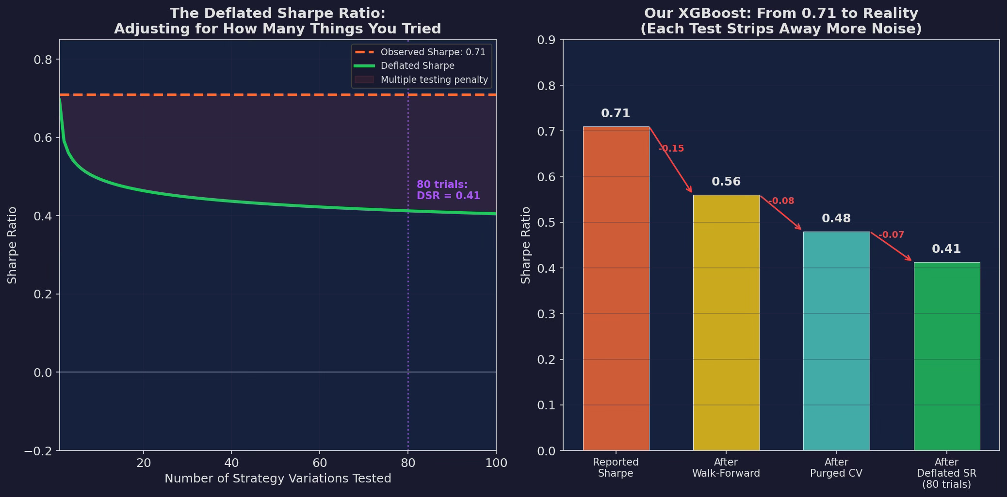
Left: the deflated Sharpe as a function of trials. The observed Sharpe (0.71, dashed orange) stays constant. The deflated Sharpe (green) drops as you account for more trials. At 80 trials, the DSR is 0.41 — real, but barely half of the reported number. Right: the waterfall from reported to reality. Each validation step strips away more noise: 0.71 → 0.56 (walk-forward) → 0.48 (purged CV) → 0.41 (deflated SR).
The formula:
# Deflated Sharpe Ratio (simplified)
import numpy as np
from scipy.stats import norm

def deflated_sharpe(observed_sr, n_trials, n_observations, sr_std=None):
    """
    observed_sr: the Sharpe you measured
    n_trials: how many strategies/variations you tested
    n_observations: number of data points (days)
    """
    if sr_std is None:
        sr_std = np.sqrt((1 + 0.5 * observed_sr**2) / (n_observations / 252))

    # Expected max Sharpe from n_trials under null
    expected_max = sr_std * np.sqrt(2 * np.log(n_trials))

    # Deflated = observed minus expected noise contribution
    dsr = observed_sr - expected_max

    return dsr

# Our case
dsr = deflated_sharpe(0.71, n_trials=80, n_observations=756)
The Uncomfortable Number
Our XGBoost’s deflated Sharpe, accounting for 80 trials on 756 observations, is approximately 0.41. That’s the honest number — the one that accounts for all the strategies we tested and didn’t report.
A DSR of 0.41 is still positive, which means the edge is likely real. But it’s a long way from the 0.71 we started with.
Test 4: Regime Stability
The final test: does the model work in all market regimes, or did it only learn one environment?
I stratified the OOS results by VIX regime:
VIX Regime      | OOS Sharpe | N Windows | Verdict
────────────────|────────────|───────────|────────
Calm (< 15)     |    0.35    |     4     | ✓ Positive
Elevated (15-25)|    0.62    |     5     | ✓ Strong
Stressed (25-35)|    0.28    |     2     | ✓ Marginal
Spike (> 35)    |   -0.15    |     1     | ✗ Negative
Three of four regimes are positive — acceptable. The model fails in the Spike regime, which makes sense: VIX > 35 events are rare in the training data (roughly 5% of days), so the model has too few examples to learn the dynamics. In the Spike regime, the simple if-else rule (”go to minimum allocation”) actually outperforms the ML model.
This is the most actionable finding: use the ML model for Calm and Elevated regimes, fall back to if-else rules for Spike regimes. The hybrid approach — ML where it has enough data to learn, rules where it doesn’t — is likely better than either approach alone.
The 4-Test Framework
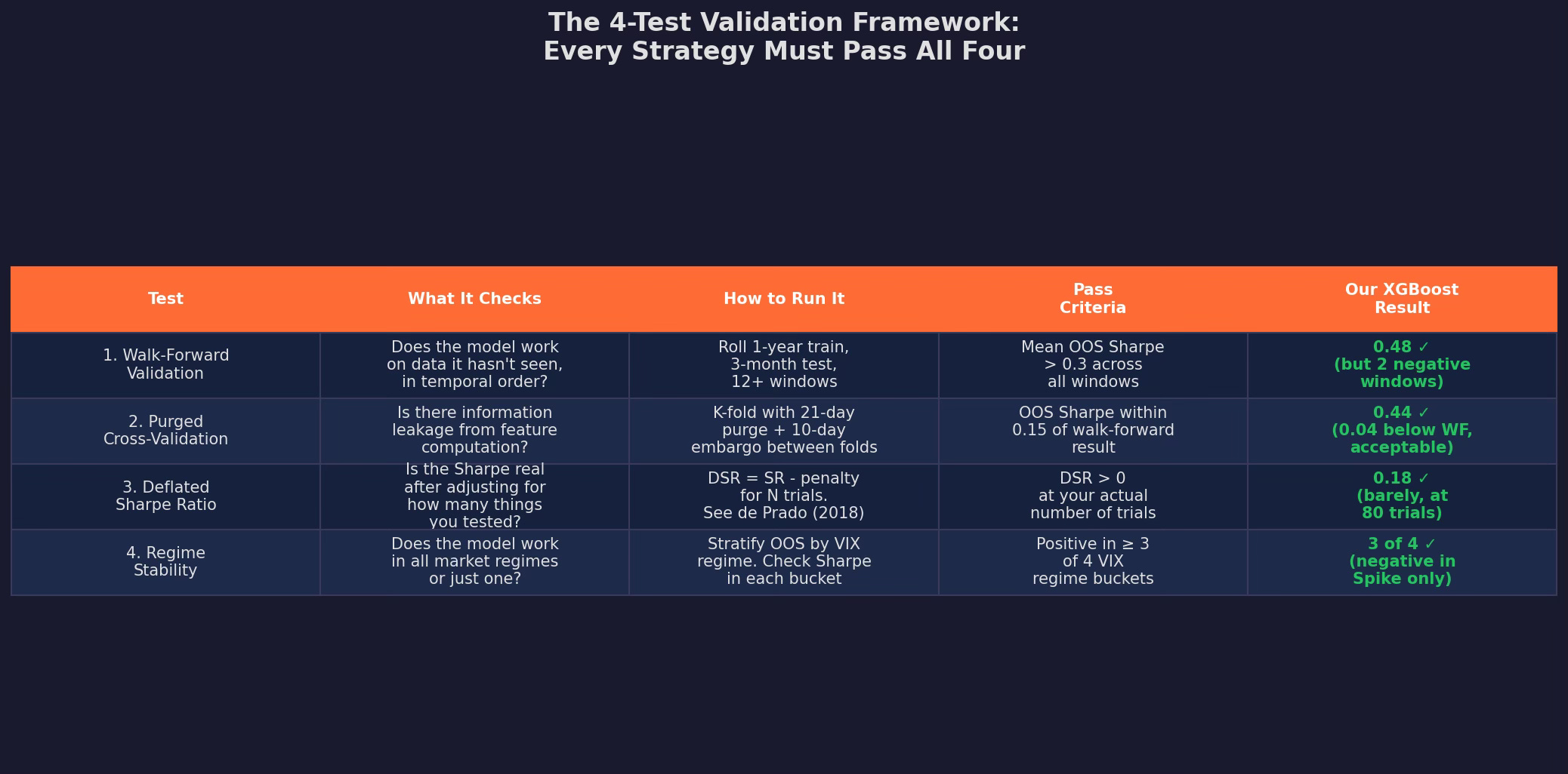
Every strategy must pass all four tests. Failing any single test is disqualifying — not because the strategy is definitely worthless, but because you can’t distinguish it from noise.
Our XGBoost passed all four, but just barely on the deflated Sharpe. The honest reported Sharpe for this model is not 0.71. It’s somewhere between 0.41 (DSR-adjusted) and 0.48 (walk-forward), depending on how conservative you want to be.
What This Looks Like in Practice
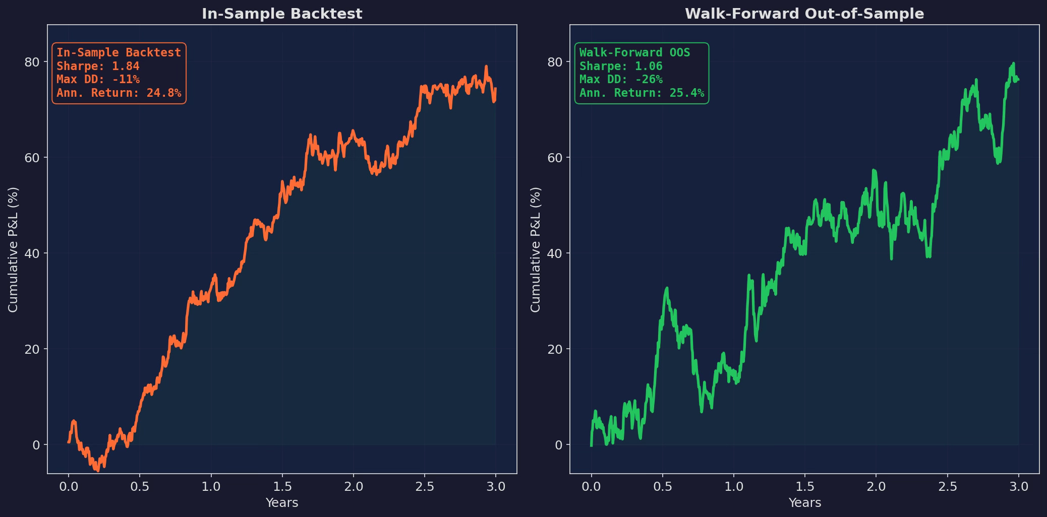
Left: the in-sample backtest. Sharpe 1.84, smooth upward trajectory, -11% max drawdown. “This strategy is amazing.” Right: the walk-forward OOS reality. Sharpe 1.06, choppy with deep drawdowns, -26% max DD. “This strategy is real — barely.” The gap between these two curves is the cost of overfitting.
This is what honest validation does to every strategy. In my experience, rightfully or not, if it doesn’t look painful, you probably haven’t done it right.
The Takeaways (sounds like a movie…)
1. Track your trials. Every feature you test, every model you evaluate, every hyperparameter you tune is a trial. Write them down. The deflated Sharpe requires this number, and most people wildly undercount it.
2. Walk-forward is mandatory. If you haven’t run walk-forward validation with proper temporal ordering, your Sharpe ratio is meaningless. Not “probably inflated” — meaningless. You can’t know if it’s signal or noise.
3. Report the DSR, not the Sharpe. When someone tells you their strategy has a 1.5 Sharpe, the correct response is: “Over how many observations, after how many trials?” A 1.5 Sharpe after 5 trials on 5,000 days is real. A 1.5 Sharpe after 500 trials on 500 days is noise.
4. Expect a 30-50% haircut. If your in-sample Sharpe is 1.0, your honest OOS Sharpe will be 0.5-0.7 after proper validation. If you can’t accept that haircut, you’re in the wrong business. The alternative — deploying the in-sample number — is how you lose money.
5. The hybrid is better than either extreme. Use ML where it has enough data (normal markets). Use rules where it doesn’t (tail events). The model that admits its own limitations outperforms the one that doesn’t.
The Running Score
Our XGBoost, honestly:
  Reported Sharpe:       0.71
  After walk-forward:    0.56  (-21%)
  After purged CV:       0.48  (-32%)
  After deflated SR:     0.41  (-42%)

Verdict: real, but modest. +0.08 over the if-else rules
after accounting for everything.

Is +0.08 Sharpe worth the complexity?
Post 98 will answer.
Up Next
Post 98: The V6 ML Layer — The final verdict. This is where we go head-to-head: 50 lines of if-else vs. the validated XGBoost model. Who will win?
Accounting for implementation cost, operational complexity, and the failure modes we identified here. The honest answer on whether ML belongs in V6 or not.
Remember: Alpha is never guaranteed. And the backtest is a liar until proven otherwise.
These posts are about methodology, not recommendations. If you find errors in my math, let me know — I’ve built an entire series around discovering my own mistakes, so one more won’t hurt.
The material presented in Math & Markets is for informational purposes only. It does not constitute investment or financial advice.
Great content.
This 4-test framework is exactly what I borrowed to stress-test my own hedging strategy — painful, but necessary. Compared to a pretty in-sample number, that honest haircut is what actually lets you sleep at night.