The Mathematics of Position Sizing, Part 2: When Kelly Goes Wrong

Part 45 — Estimation error, fat tails, and why the “optimal” bet size might blow you up

This is part 45 of my series — Building & Scaling Algorithmic Trading Strategies

---

This is a 3-part series on the mathematics of position sizing:

• Part 1: The Kelly Criterion from First Principles

• Part 2: When Kelly Goes Wrong (estimation error, fat tails, non-ergodicity)

• Part 3: Practical Kelly (fractional Kelly, multi-asset, constraints)

---

The Problem With Being “Optimal”

In Part 1, I derived the Kelly Criterion and showed it maximizes long-run growth. The formula is elegant:

f* = (μ - r) / σ²

For SPY with μ = 10%, r = 5%, σ = 16%, Kelly recommended 195% leverage.

That number should make you uncomfortable. If it doesn’t, this post will fix that.

Kelly is optimal in theory. In practice, it’s a recipe for disaster unless you understand exactly where the math breaks down.

---

1. The Estimation Problem

Kelly requires knowing μ and σ. We don’t know them. We estimate them.

Let’s see what happens when estimates are wrong.

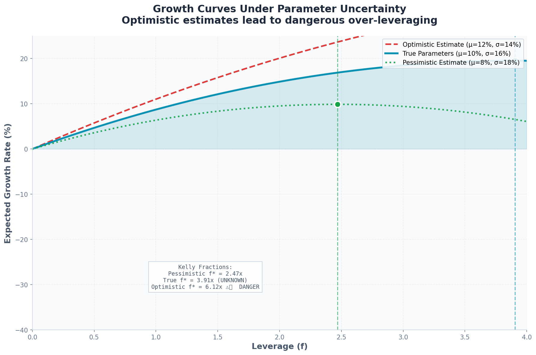
The Setup

True parameters (unknown to us):

• μ = 10%

• σ = 16%

• True Kelly: f* = 0.05 / 0.0256 = 1.95

Our estimates (from historical data):

• μ̂ = 12% (we’re 2% too optimistic)

• σ̂ = 14% (we’re underestimating vol)

• Estimated Kelly: f̂* = 0.07 / 0.0196 = 3.57

We think we should use 3.57x leverage. True optimal is 1.95x.

The Cost of Overestimation

The growth rate under Kelly betting is:

g(f) = μf - (σ²f²)/2

If we bet f̂* = 3.57 but true parameters are μ = 10%, σ = 16%:

g(3.57) = 0.10 × 3.57 - (0.0256 × 3.57²) / 2
        = 0.357 - 0.163
        = 0.194  (19.4% growth)

Compare to true Kelly:

g(1.95) = 0.10 × 1.95 - (0.0256 × 1.95²) / 2
        = 0.195 - 0.049
        = 0.146  (14.6% growth)

Wait—the overestimated Kelly still grows faster?

Not so fast. That’s the expected growth rate. The variance of growth matters too.

Variance of Growth

The variance of log returns scales with f²σ²:

Var[log return] = f²σ²

At f = 3.57: Variance = 3.57² × 0.0256 = 0.326 At f = 1.95: Variance = 1.95² × 0.0256 = 0.097

The overestimated position has 3.4x higher variance.

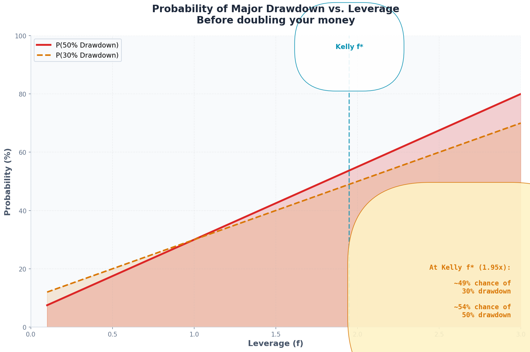
Probability of Drawdown

With higher variance comes higher probability of catastrophic loss.

For a given time horizon T, the probability of experiencing a drawdown of size D or worse:

P(max drawdown ≥ D) ≈ 2Φ(-D / (σf√T))

For a 50% drawdown over 1 year:

• f = 1.95: P(DD ≥ 50%) ≈ 5.2%

• f = 3.57: P(DD ≥ 50%) ≈ 18.7%

Overestimating Kelly triples your probability of catastrophic loss.

---

2. The Asymmetry of Error

Here’s something Kelly practitioners learn the hard way: Overestimating f is worse than underestimating.*

The growth function g(f) is:

g(f) = μf - (σ²f²)/2

This is a downward-opening parabola. The Kelly point f* = μ/σ² is the peak.

The Shape Matters

Near the peak, small errors in either direction cost you a little growth. But the function falls off asymmetrically.

Specifically, the second derivative:

d²g/df² = -σ²

This is constant and negative—so the parabola is symmetric in f. But growth is exponential, not linear. A 5% reduction in growth rate costs more over time than you’d naively expect.

More importantly: Over-betting can push you past the ruin boundary.

If you bet f > 2/a (where a is the loss fraction), you can go broke on a single bad outcome.

For our coin flip example (a = 0.5):

• Ruin boundary: f > 2/0.5 = 4.0 (400% bet)

With f = 3.57, you’re not at ruin yet. But you’re close. And estimation error is symmetric—you could just as easily estimate f̂* = 4.5.

The Rule of Thumb

Because overestimation is more dangerous than underestimation, the rational response to parameter uncertainty is to bet less than your point estimate.

This leads directly to fractional Kelly, which we’ll cover in Part 3.

---

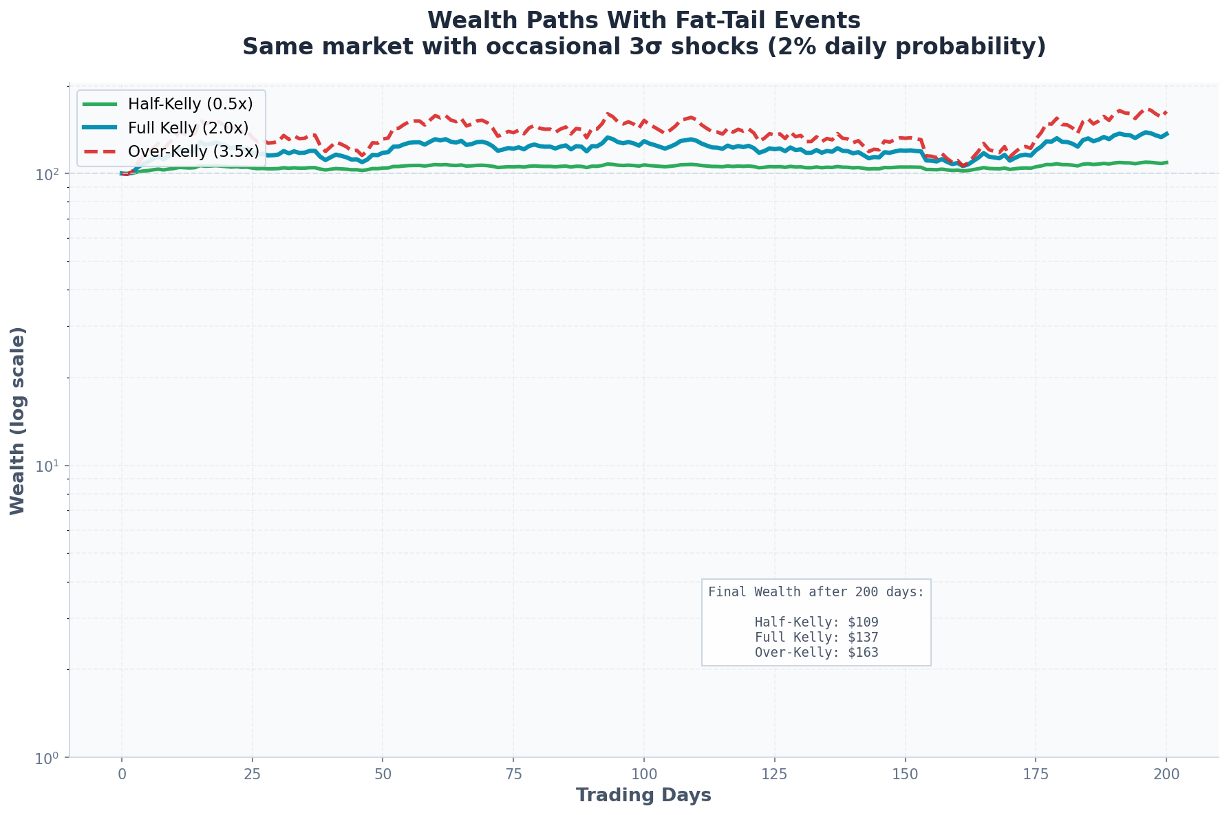
3. Fat Tails: When Variance Isn’t Enough

Kelly assumes returns are normally distributed (or at least have finite variance). Markets don’t oblige.

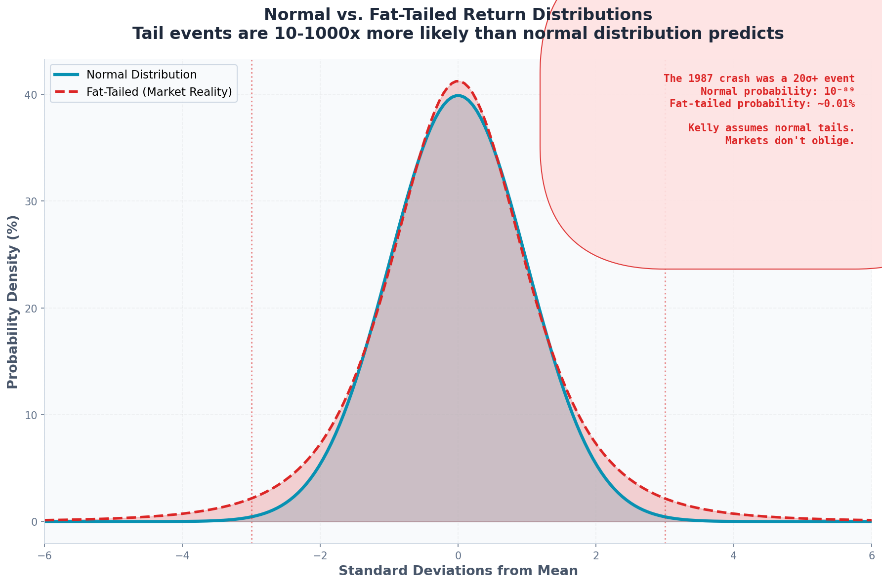
The Problem

Normal distribution:

P(|X| > 3σ) ≈ 0.27%
P(|X| > 5σ) ≈ 0.00006%

Actual market returns (S&P 500):

P(|X| > 3σ) ≈ 1.5%      (6x more frequent)
P(|X| > 5σ) ≈ 0.1%      (1,600x more frequent)

The 1987 crash was a 20+ sigma event under normal assumptions. The probability of that occurring by chance: 10^(-89).

It happened.

How Fat Tails Break Kelly

Kelly optimizes expected log growth:

E[ln(W_new)] = E[ln(W(1 + fR))]

For small f and normally distributed R, this expands to:

E[ln(W_new)] ≈ ln(W) + fμ - f²σ²/2

But this Taylor expansion assumes higher moments are negligible. With fat tails, they’re not.

The full expansion:

E[ln(1 + fR)] = fμ - f²σ²/2 + f³κ₃/6 - f⁴κ₄/24 + ...

Where κ₃ (skewness) and κ₄ (kurtosis) are the higher moments.

For fat-tailed distributions, κ₄ >> 3 (normal has κ₄ = 3). This means the f⁴ term penalizes large bets more than the standard Kelly formula suggests.

Fat-Tail Adjusted Kelly

One practical adjustment: replace σ² with a “tail-adjusted” variance that accounts for kurtosis:

σ²_adj = σ² × (1 + (κ₄ - 3) / (4 + 2(κ₄ - 3)))

For SPY with excess kurtosis around 3-5:

σ²_adj = 0.0256 × (1 + 4/10) = 0.0358

This drops the Kelly fraction from 1.95 to:

f*_adj = 0.05 / 0.0358 = 1.40

A 28% reduction just from acknowledging fat tails.

---

4. Non-Ergodicity: Why Your Path Matters

This is where things get philosophically interesting.

The Ergodicity Assumption

Kelly’s proof that it “beats everything over time” relies on an ergodic assumption: the time-average of your wealth equals the ensemble average.

In simpler terms: what happens to you over many trials equals what would happen to the average of many “you”s over one trial.

For coin flips, this holds perfectly. For financial markets, it does not.

Why Markets Are Non-Ergodic

Consider two scenarios with identical expected returns:

Scenario A: Gaussian returns with μ = 10%, σ = 16%

Scenario B: 99% chance of +11%, 1% chance of -80%

Both have E[R] ≈ 10%. Both have similar variance. But:

• In Scenario A, any given year is “typical”

• In Scenario B, most years are great, but one year ruins you

The Kelly formula treats these identically. Your lived experience does not.

The Absorbing Barrier Problem

Once your wealth hits zero, you’re out. You can’t recover.

Kelly assumes continuous rebalancing with infinitely divisible wealth. Reality includes:

• Margin calls

• Minimum account balances

• Psychological breaking points

• Leverage constraints that tighten during drawdowns

These create “absorbing barriers” that the theoretical Kelly ignores.

The Mathematics of Ruin

For a leveraged position with drawdown threshold D, the probability of hitting that threshold before doubling is:

P(ruin before double) = (e^(2μD/σ²) - 1) / (e^(2μD/σ²) - e^(-2μ/σ²))

For Kelly-optimal leverage (f* = μ/σ²) with D = 50%:

P(50% DD before 100% gain) ≈ 28%

That’s not a tail event.

That’s a one-in-four chance of losing half your money before you double it.

---

5. Regime Changes: When Parameters Shift

Kelly assumes stationarity. The game stays the same forever.

Markets don’t work that way.

The V6 Reminder

In my V6 Dual Allocator work, I found that VIX regimes completely change the game:

VIX Regime    TQQQ Return    Optimal Leverage
< 15          +148%          High
15-25         +60%           Moderate
25-35         -41%           Zero or negative
> 35          -539%          Definitely zero

A Kelly fraction calibrated to the full sample is meaningless when the parameters swing from +148% to -539% depending on regime.

Conditional Kelly

The solution is regime-conditional Kelly:

f*(regime) = (μ_regime - r) / σ²_regime

Low VIX regime:

• μ = 40%, σ = 20%

• f* = 0.35 / 0.04 = 8.75 (!)

High VIX regime:

• μ = -30%, σ = 50%

• f* = -0.35 / 0.25 = -1.40 (short!)

This matches the intuition in V6: be aggressive when volatility is low, defensive (or short) when it’s high.

But now you need to:

1. Correctly identify the current regime

2. Estimate μ and σ for each regime

3. Handle transitions between regimes

Each step introduces additional estimation error.

---

6. The Leverage Decay Problem

With leveraged ETFs (like TQQQ in my V6 strategy), there’s an additional wrinkle: volatility decay.

Daily Rebalancing Kills You

A 3x leveraged ETF rebalances daily to maintain 3x exposure. This creates path dependency.

Consider QQQ over two days:

Day 1: +10% Day 2: -10%

QQQ: $100 → $110 → $99 (-1%) TQQQ: $100 → $130 → $91 (-9%)

TQQQ lost 9%, not 3%. This is volatility decay (or “beta slippage”).

The Decay Formula

For a leveraged ETF with leverage L and underlying volatility σ over horizon T:

Expected decay = L × (L-1) × σ² × T / 2

For TQQQ (L = 3) with σ = 20% annualized over 1 year:

Decay = 3 × 2 × 0.04 × 1 / 2 = 0.12 (12% annual decay)

This 12% drag comes straight off your returns.

Kelly for Leveraged ETFs

The Kelly formula needs adjustment:

f*_lev = (μ_underlying × L - decay - r) / (σ_underlying × L)²

For QQQ:

• μ_underlying = 15%

• σ_underlying = 20%

• L = 3 (TQQQ)

• decay = 12%

• r = 5%

f*_TQQQ = (0.15 × 3 - 0.12 - 0.05) / (0.20 × 3)²
        = (0.45 - 0.17) / 0.36
        = 0.28 / 0.36
        = 0.78

Kelly says only 78% allocation to TQQQ, even in favorable conditions.

Compare to unleveraged QQQ:

f*_QQQ = (0.15 - 0.05) / 0.04 = 2.50

The volatility decay of TQQQ is severe enough that Kelly prefers 250% leveraged QQQ over 78% TQQQ.

(This partly vindicates V6’s regime-switching. When VIX is high, decay accelerates, and even small TQQQ allocations become negative Kelly.)

---

7. The Behavioral Barrier

Everything above assumes you execute the strategy faithfully. You won’t.

Prospect Theory vs. Kelly

Kahneman and Tversky showed that humans:

• Feel losses 2-2.5x more intensely than equivalent gains

• Are risk-seeking in losses, risk-averse in gains

• Anchor to recent experience

Kelly betting creates experiences that violate all of these:

• Large, frequent drawdowns (feels 2x worse than it “should”)

• Requires staying the course during losses (impossible for loss-averse humans)

• Ignores recent experience (no adjustment for “this feels wrong”)

The Drawdown Experience

At Kelly-optimal sizing, expected max drawdown over time horizon T is roughly:

E[max DD] ≈ σ√T × f* / √2

For f* = 2.0 and σ = 16% over 10 years:

E[max DD] ≈ 0.16 × 3.16 × 2.0 / 1.41 = 72%

Can you hold through a 72% drawdown? Most can’t. The ones who say they can haven’t tried.

The Sequence of Returns Problem

Even with correct sizing, the order of returns matters for your psychological state.

Simulation A: Lose 30% in year 1, then grow steadily Simulation B: Grow steadily for 9 years, lose 30% in year 10

Mathematically identical. Psychologically, B feels like “giving back gains” and A feels like “the strategy doesn’t work.”

Both conclusions are wrong. But you’ll feel them anyway.

---

8. What This Means for Position Sizing

Let’s tally the adjustments Kelly needs:

Factor Adjustment to f* Estimation error −20% to −50% Fat tails −20% to −40% Regime uncertainty Regime-conditional Leverage decay Depends on L Behavioral tolerance −50% or more

Stacking these conservatively:

• Start with theoretical f* = 1.95

• Estimation error: × 0.7 = 1.37

• Fat tails: × 0.75 = 1.03

• Behavioral tolerance: × 0.5 = 0.51

Adjusted Kelly: 51% allocation instead of 195%.

That’s a 74% reduction from the “optimal” value.

---

9. The Fractional Kelly Preview

This leads naturally to fractional Kelly—betting some fraction of the Kelly amount:

f_actual = c × f*

Where c ∈ (0, 1) is the “Kelly fraction.”

Common choices:

• c = 0.5 (”half-Kelly”): Most popular in practice

• c = 0.25 (”quarter-Kelly”): Very conservative

• c = 0.1: Barely distinguishable from constant-fraction betting

In Part 3, we’ll derive the optimal c given uncertainty in parameters, show how fractional Kelly affects the growth-drawdown tradeoff, and build a practical framework for multi-asset Kelly allocation.

---

10. Summary: The Kelly Failure Modes

Kelly goes wrong when:

1. You don’t know μ and σ — Estimation error compounds; overestimation is especially dangerous

2. Returns have fat tails — Higher moments penalize large bets; standard Kelly underestimates risk

3. Markets are non-ergodic — You only get one path; ruin is absorbing; time averages ≠ ensemble averages

4. Regimes shift — Full-sample parameters are meaningless when μ flips sign

5. Leverage decays — Volatility drag creates hidden costs that standard Kelly ignores

6. You’re human — Drawdowns hurt more than gains help; you’ll abandon the strategy at the worst time

The theoretical optimality of Kelly is mathematically beautiful and practically useless without adjustments.

---

The Bottom Line

Kelly is a ceiling, not a target.

The formula tells you the maximum bet you should ever consider—and only under idealized assumptions. In reality, you should bet substantially less.

The question isn’t “what does Kelly say?” It’s “how much less than Kelly should I bet given my uncertainty?”

That’s what Part 3 will answer.

---

In Part 3: Practical Kelly — fractional Kelly derivation, multi-asset allocation, and a position sizing framework you can actually use.

---

This post is about methodology, not recommendations. Position sizing decisions depend on individual circumstances. The Kelly criterion can suggest leveraged positions that may be inappropriate for most investors. If you find errors in my math, let me know.

The information presented in Math & Markets is not investment or financial advice and should not be construed as such.

---