The Mathematics of Position Sizing, Part 3: Practical Kelly

Part 46 — Fractional Kelly, multi-asset allocation, and a framework you can actually use

This is part 46 of my series — Building & Scaling Algorithmic Trading Strategies

---

This is a 3-part series on the mathematics of position sizing:

• Part 1: The Kelly Criterion from First Principles

• Part 2: When Kelly Goes Wrong (estimation error, fat tails, non-ergodicity)

• Part 3: Practical Kelly (fractional Kelly, multi-asset, constraints)

---

Part 1 derived Kelly. Part 2 broke it.

Now we rebuild. The goal: a position sizing framework that captures Kelly’s insights without its pathologies.

The key realization is that Kelly isn’t a formula to follow blindly — it’s an upper bound on reasonable bet sizes. What we actually need is a systematic way to stay below that bound while preserving most of the growth benefit.

---

1. Fractional Kelly: The Core Idea

Fractional Kelly is simple: bet a fraction of the Kelly amount.

f_actual = c × f*

Where c ∈ (0, 1) is the “Kelly fraction.”

The Tradeoff

Fractional Kelly trades off expected growth for reduced variance and drawdown.

For a full Kelly bet, expected growth is:

g* = μ²/(2σ²) = SR²/2

For fractional Kelly at fraction c:

g(c) = c × μ × f* - (c² × σ² × f*²)/2
     = c × g* × (2 - c)

Normalizing by full Kelly growth:

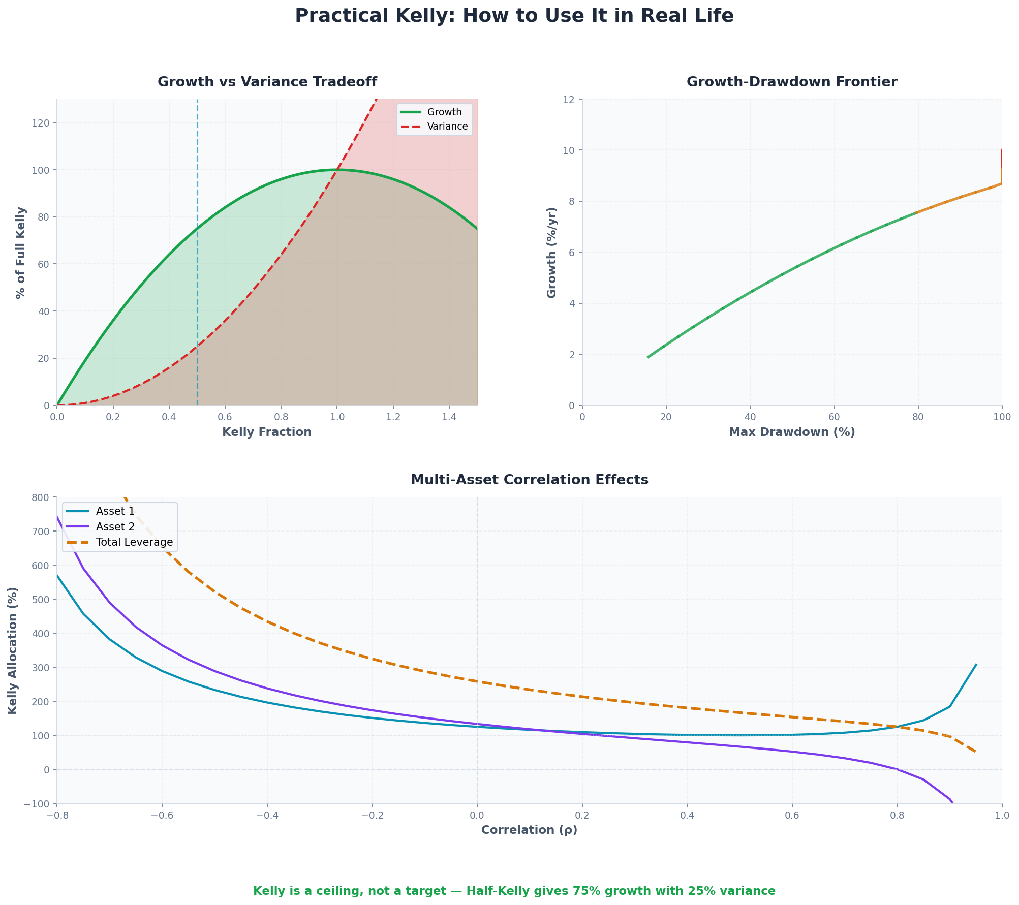
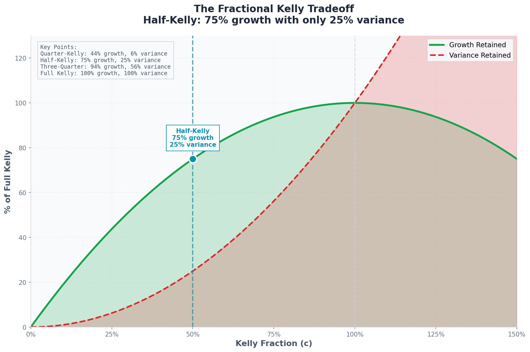
g(c)/g* = c(2 - c)

This is a remarkable result. Let’s tabulate:

Kelly Fraction (c) Growth Ratio Variance Ratio 1.00 (Full) 100% 100% 0.75 94% 56% 0.50 (Half) 75% 25% 0.25 (Quarter) 44% 6% 0.10 19% 1%

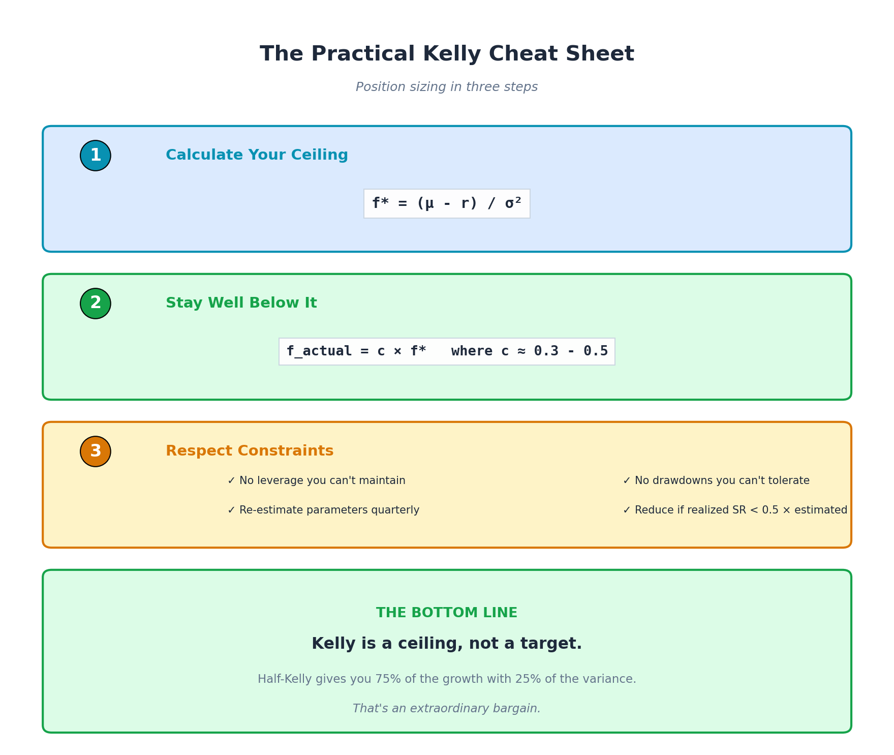
Half-Kelly gives you 75% of the growth with 25% of the variance.

This is an extraordinary bargain. You sacrifice one quarter of your long-run growth to eliminate three quarters of your volatility.

---

2. Optimal Fractional Kelly Under Uncertainty

Part 2 showed that parameter uncertainty is the main practical problem. Can we derive the optimal Kelly fraction given estimation error?

The Setup

Let:

• μ̂, σ̂ = estimated parameters

• μ, σ = true parameters (unknown)

• f̂* = μ̂/σ̂² = estimated Kelly fraction

• f* = μ/σ² = true Kelly fraction

We want to choose c to maximize expected growth, accounting for the fact that f̂* ≠ f*.

Estimation Error Model

Assume our estimates have multiplicative errors:

μ̂ = μ × (1 + ε_μ)
σ̂ = σ × (1 + ε_σ)

Where ε_μ and ε_σ are zero-mean random variables with standard deviations δ_μ and δ_σ.

Then the ratio of estimated to true Kelly:

f̂*/f* = (1 + ε_μ) / (1 + ε_σ)²

For small errors, this approximates:

f̂*/f* ≈ 1 + ε_μ - 2ε_σ

The variance of this ratio:

Var[f̂*/f*] ≈ δ_μ² + 4δ_σ²

The Optimal Fraction

Given estimation uncertainty, the optimal Kelly fraction is approximately:

c* = 1 / (1 + Var[f̂*/f*])

This is a beautiful result. If you have no estimation error, c* = 1 (full Kelly). As estimation error increases, c* decreases.

Numerical Example

Suppose:

• δ_μ = 30% (you could be 30% off on expected return)

• δ_σ = 15% (you could be 15% off on volatility)

Var[f̂*/f*] ≈ 0.30² + 4 × 0.15² = 0.09 + 0.09 = 0.18

c* = 1 / (1 + 0.18) = 1 / 1.18 = 0.85

With typical estimation uncertainty, optimal Kelly fraction is around 0.85.

But wait — this assumes your errors are unbiased. I mean, that’s a rather rich assumption. In practice, people systematically overestimate returns and underestimate volatility. I certainly do! So adding a bias correction pushes c* lower, often to 0.5 - 0.7.

---

3. The Drawdown-Growth Frontier

Another way to choose c: specify your maximum acceptable drawdown, then solve for the corresponding Kelly fraction.

Maximum Drawdown Formula

For Kelly betting with fraction c, the expected maximum drawdown over time horizon T is approximately:

E[MDD] ≈ c × σ × √(2T) × f* / √π

For continuous returns, this simplifies to:

E[MDD] ≈ c × √(2 × g* × T / π)

Where g* is the full-Kelly growth rate.

Example: Targeting 25% Max Drawdown

Say you want E[MDD] ≤ 25% over a 10-year horizon.

With full-Kelly growth g* = 10% (SR ≈ 0.45):

0.25 ≈ c × √(2 × 0.10 × 10 / π)
0.25 ≈ c × √(0.637)
0.25 ≈ c × 0.80
c ≈ 0.31

To keep expected drawdown under 25%, you need Kelly fraction of ~0.31.

The Frontier

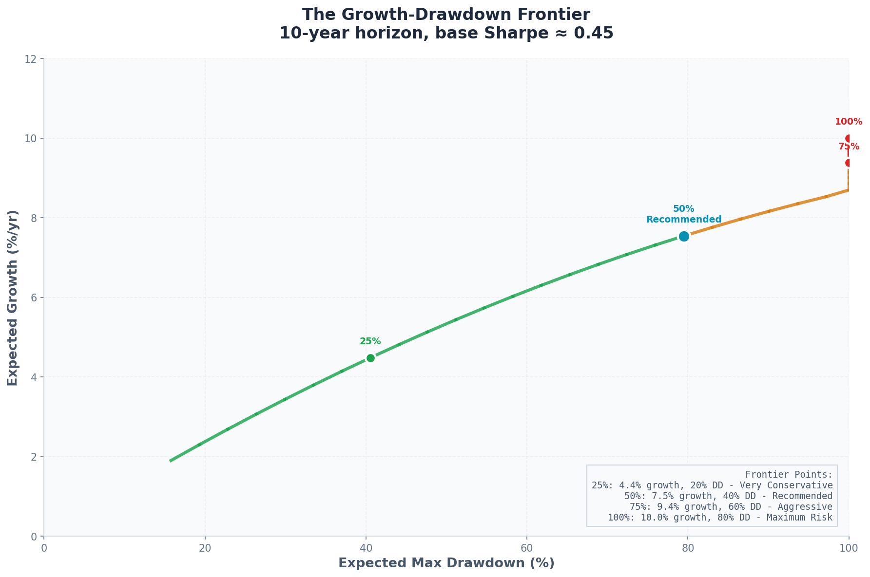
You can trace out the full frontier of growth vs. drawdown:

Kelly Fraction Expected Growth Expected Max DD (10yr) 1.00 10.0% 80% 0.75 9.4% 60% 0.50 7.5% 40% 0.35 5.8% 28% 0.25 4.4% 20%

This frontier makes the tradeoff concrete. Full Kelly gives you 10% growth but 80% expected drawdown. Quarter-Kelly gives you 4.4% growth but only 20% drawdown.

---

4. Multi-Asset Kelly: The General Case

Real portfolios have multiple assets. Kelly generalizes to this case, but the math gets more interesting.

The Multi-Asset Problem

With n assets, the Kelly problem becomes:

Maximize: E[ln(1 + f’R)]
Subject to: Σf_i ≤ 1 (or leverage constraint)

Where:

• f = (f₁, f₂, ..., fₙ) is the vector of allocations

• R = (R₁, R₂, ..., Rₙ) is the vector of returns

• f’R = Σf_i × R_i is the portfolio return

The Solution

For normally distributed returns with mean vector μ and covariance matrix Σ:

f* = Σ⁻¹(μ - r1)

Where r is the risk-free rate and 1 is a vector of ones.

This is the same as the mean-variance optimal portfolio with risk aversion λ = 1.

Why Correlation Matters

The Kelly allocation to asset i depends on all the other assets through the inverse covariance matrix.

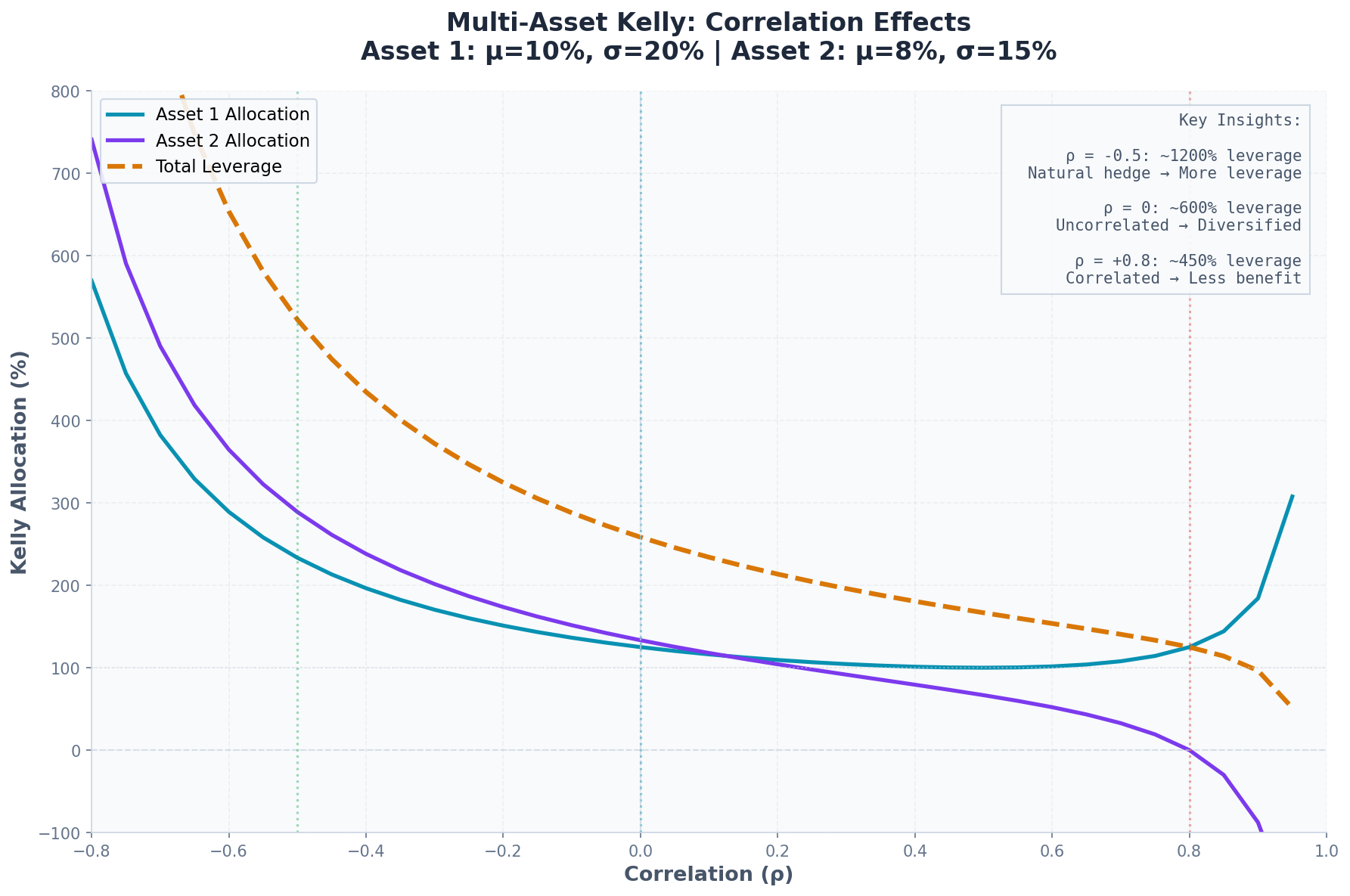
Consider two assets with:

• μ₁ = 10%, σ₁ = 20%

• μ₂ = 8%, σ₂ = 15%

• Correlation ρ

Case 1: ρ = 0 (uncorrelated)

Σ = [0.04   0   ]
    [0      0.0225]

Σ⁻¹ = [25      0    ]
      [0       44.4  ]

f* = Σ⁻¹μ = [25 × 0.10,  44.4 × 0.08]
          = [2.50,  3.55]

Kelly says: 250% in Asset 1, 355% in Asset 2. That’s 6x leverage total.

Case 2: ρ = 0.8 (highly correlated)

Σ = [0.04    0.024 ]
    [0.024   0.0225]

Σ⁻¹ = [89.3   -95.2]
      [-95.2  159.7]

f* = [89.3×0.10 - 95.2×0.08,  -95.2×0.10 + 159.7×0.08]
   = [8.93 - 7.62,  -9.52 + 12.78]
   = [1.31,  3.26]

Now Kelly says: 131% in Asset 1, 326% in Asset 2. Still leveraged, but the high correlation reduces the diversification benefit and hence the total allocation.

Case 3: ρ = -0.5 (negatively correlated)

Σ⁻¹ = [33.3   22.2]
      [22.2   53.3]

f* = [33.3×0.10 + 22.2×0.08,  22.2×0.10 + 53.3×0.08]
   = [3.33 + 1.78,  2.22 + 4.26]
   = [5.11,  6.48]

Kelly says: 511% in Asset 1, 648% in Asset 2. Negative correlation creates a natural hedge, so Kelly recommends more leverage.

The Practical Problem

Multi-asset Kelly requires estimating the full covariance matrix Σ. With n assets, that’s n(n+1)/2 parameters — far more estimation error than the single-asset case.

For n = 10 assets: 55 parameters to estimate and or n = 100 assets: 5,050 parameters — as you can see, the estimation error problem explodes!

---

5. Shrinkage and Robust Estimation

The standard solution to estimation error in multi-asset Kelly: shrinkage estimators.

The Idea

Instead of using raw sample estimates, blend them toward a simpler model:

μ̂_shrunk = (1-α) × μ̂_sample + α × μ_prior
Σ̂_shrunk = (1-β) × Σ̂_sample + β × Σ_prior

Where:

• α, β ∈ (0,1) are shrinkage intensities

• μ_prior, Σ_prior are “prior” estimates (often the market portfolio or identity matrix)

Ledoit-Wolf Shrinkage

The most common approach for covariance estimation is Ledoit-Wolf, which shrinks toward a scaled identity matrix:

Σ̂_LW = (1-δ) × Σ̂_sample + δ × (trace(Σ̂)/n) × I

The optimal δ minimizes expected squared error and can be computed from the data.

Typical values: δ ≈ 0.3-0.5 for sample sizes around 100-500.

Effect on Kelly

Shrinkage reduces the extreme allocations that arise from covariance estimation error.

Without shrinkage, Kelly might say: [300%, -150%, 250%, -50%, ...] With shrinkage, Kelly might say: [80%, 20%, 60%, 10%, ...]

The second is more plausible and more robust.

Rule of Thumb

If n/T > 0.1 (number of assets divided by number of time periods), shrinkage is essential. Below that threshold, sample estimates might be acceptable.

For practical portfolios with 10-50 assets and 5-10 years of monthly data (60-120 observations), shrinkage is always necessary.

---

6. The Practical Framework

Let me synthesize everything into a usable position sizing framework.

Step 1: Estimate Parameters

For each asset or strategy:

1. Calculate sample mean (μ̂) and volatility (σ̂) from historical data

2. Apply shrinkage toward reasonable priors (market portfolio, long-term averages)

3. For multiple assets, use Ledoit-Wolf or similar for covariance estimation

Step 2: Calculate Raw Kelly

Single asset:

f̂* = (μ̂ - r) / σ̂²

Multiple assets:

f̂* = Σ̂⁻¹(μ̂ - r1)

Step 3: Apply Fractional Kelly

Choose your Kelly fraction c based on:

• Estimation uncertainty: c = 1/(1 + estimation_variance), typically 0.5-0.8

• Drawdown tolerance: Use the frontier table to map target drawdown to c

• Behavioral realism: Can you actually hold through the drawdowns? If not, reduce c

Recommended starting point: c = 0.5 (half-Kelly)

Step 4: Apply Constraints

Real portfolios have constraints:

• Leverage limits: f_total ≤ L_max

• Position limits: f_i ≤ f_max for all i

• Sector limits: Sum of positions in sector ≤ s_max

• Long-only: f_i ≥ 0 for all i

Solve the constrained optimization:

Maximize: E[ln(1 + f’R)]
Subject to: constraints

This usually requires numerical optimization (quadratic programming).

Step 5: Regime Adjustment

From my V6 work, we know that parameters change across regimes. The framework should adjust:

Low VIX regime (VIX < 20):

• Use μ, σ estimates from calm periods

• Apply standard Kelly fraction

High VIX regime (VIX > 30):

• Use μ, σ estimates from volatile periods

• Reduce Kelly fraction further (c → c/2)

• Or switch to defensive assets (TLT in V6)

Step 6: Rebalancing

Kelly assumes continuous rebalancing, which is impractical. Choices:

• Calendar rebalancing: Monthly or quarterly

• Threshold rebalancing: When position drifts >20% from target

• Volatility-triggered: Rebalance when VIX crosses regime thresholds

Each approach has tradeoffs between transaction costs and tracking error.

---

7. A Worked Example: The V6 Dual Allocator

Let me apply this framework to my V6 strategy.

The Assets

• TQQQ: μ ≈ 35% (in favorable regime), σ ≈ 60%

• QQQ: μ ≈ 15%, σ ≈ 20%

• TLT: μ ≈ 4%, σ ≈ 15%

• Cash: μ = 5%, σ = 0%

Raw Kelly Calculations

TQQQ (low VIX regime):

f*_TQQQ = (0.35 - 0.05) / 0.36 = 0.83

QQQ:

f*_QQQ = (0.15 - 0.05) / 0.04 = 2.50

TLT:

f*_TLT = (0.04 - 0.05) / 0.0225 = -0.44

Raw Kelly says: 83% TQQQ, 250% QQQ (or short 44% TLT as a funding vehicle).

Apply Fractional Kelly (c = 0.5)

f_TQQQ = 0.5 × 0.83 = 0.42 (42%)
f_QQQ = 0.5 × 2.50 = 1.25 (125%)

Still implies leverage, but less extreme.

Apply Constraints

Constraint: No leverage (f_total ≤ 1)

Normalize:

f_TQQQ = 0.42 / 1.67 = 25%
f_QQQ = 1.25 / 1.67 = 75%

Or, given the leverage inside TQQQ (3x), we might prefer:

f_TQQQ = 33% (equivalent to 100% leveraged QQQ exposure)
f_QQQ = 67%

V6’s Actual Allocation

V6 uses:

• 100% TQQQ in strong uptrends with low VIX

• 70% TQQQ in moderate conditions

• 100% TLT in high VIX

How does this compare to the Kelly framework?

In low VIX strong uptrend:

• Kelly-optimal TQQQ allocation: ~83% (unconstrained), ~42% (half-Kelly)

• V6 allocation: 100%

V6 is over-betting relative to half-Kelly.

But V6 compensates with regime switching. It’s not 100% TQQQ all the time — it’s 100% conditional on being in a favorable regime. This is closer to conditional Kelly.

Refinement Suggestion

Based on this analysis, V6 could potentially be improved by:

1. Reducing max TQQQ allocation from 100% to 70%

2. Adding a 30% QQQ or TLT position even in favorable regimes

3. Increasing the VIX threshold for full TQQQ from <15 to <12

This would reduce variance without much growth sacrifice.

---

8. The Position Sizing Checklist

Here’s a practical checklist for any new strategy:

Before implementing:

• [ ] Calculate raw Kelly fraction from backtest parameters

• [ ] Apply half-Kelly (or less) as a starting point

• [ ] Check that position size survives 2x the max historical drawdown

• [ ] Ensure leverage (if any) is within broker/regulatory limits

Ongoing:

• [ ] Re-estimate parameters quarterly

• [ ] Track actual vs. expected Sharpe ratio

• [ ] If realized Sharpe < 0.5 × estimated, reduce position size

• [ ] Monitor regime indicators (VIX, trend)

• [ ] Rebalance on schedule or at thresholds

Red flags:

• [ ] Position size implies >3x leverage → Reduce

• [ ] Estimated Sharpe > 2.0 → Be skeptical

• [ ] Backtest parameters from <3 years → Insufficient data

• [ ] Strategy requires precision timing → Likely overfit

---

9. What Kelly Teaches (Even If You Don’t Use It)

Even if you never calculate a Kelly fraction, the framework teaches important lessons:

1. Position size matters as much as strategy: Two traders with identical signals but different position sizing will have completely different outcomes. Kelly makes this explicit.

2. There’s a maximum reasonable bet: No edge justifies unlimited leverage. Kelly provides a principled upper bound.

3. Volatility is a tax: The Kelly formula shows exactly how volatility reduces growth. This justifies volatility targeting and regime-switching.

4. Estimation error compounds: Errors in μ and σ don’t just cause proportional errors in f* — they can flip the sign. This justifies conservative sizing.

5. Diversification works (if correlations are right): Multi-asset Kelly shows how uncorrelated bets can support more leverage than concentrated ones.

6. Drawdowns are features, not bugs: Kelly-optimal sizing implies substantial drawdowns. If you can’t tolerate them, you’re either over-betting or under-compensated for risk.

---

10. Summary: The Practical Kelly Framework

Position sizing in three steps:

Step 1: Calculate your ceiling

f* = (μ - r) / σ²  or  f* = Σ⁻¹(μ - r)

Step 2: Stay well below it

f_actual = c × f*  where c ≈ 0.3-0.5

Step 3: Respect constraints

• No leverage you can’t maintain

• No drawdowns you can’t tolerate

• No estimation errors you haven’t hedged

---

Conclusion: The Position Sizing Series

Over three posts, we’ve covered:

Part 1: The Kelly Criterion derivation and why it maximizes long-run growth

Part 2: Why Kelly fails in practice — estimation error, fat tails, non-ergodicity, regime changes, and behavioral limits

Part 3: How to use Kelly practically — fractional Kelly, multi-asset allocation, and a usable framework

The core insight: Kelly isn’t a formula to follow — it’s a framework for thinking about position sizing. It tells you the maximum you should ever consider betting, and provides tools for systematically betting less.

For my own trading, the implications are:

• V6’s 100% TQQQ allocation is aggressive but defensible given regime switching

• Adding a fractional Kelly layer could reduce volatility without much growth sacrifice

• The TLT hedge in high-VIX regimes is Kelly-consistent (switching to a different game)

Position sizing is the least glamorous part of systematic trading — it doesn’t generate alpha and it doesn’t find new signals. However, it does help determine whether your signals survive long enough to matter. And Kelly gives you a language for that conversation!

---

End of the Position Sizing Series. Next: something new.

This post is about methodology, not recommendations. Position sizing decisions depend on individual circumstances I don’t know. If you find errors in my math, let me know.

The information presented in Math & Markets is not investment or financial advice and should not be construed as such.

---