The Mathematics of Position Sizing, Part 1: The Kelly Criterion from First Principles

Part 44 — What a 1956 Bell Labs paper teaches us about bet sizing

This is part 44 of my series — Building & Scaling Algorithmic Trading Strategies

---

This is a 3-part series on the mathematics of position sizing:

• Part 1: The Kelly Criterion from First Principles

• Part 2: When Kelly Goes Wrong (estimation error, fat tails, non-ergodicity)

• Part 3: Practical Kelly (fractional Kelly, multi-asset, constraints)

---

The Problem Nobody Talks About

I’ve spent 43 posts obsessing over what to trade. Momentum signals. Volatility regimes. VIX thresholds. TLT hedges. Options. Synthetic Data. Satellite Imagery.

But I’ve mostly hand-waved how much to trade.

V6 allocates 100% to TQQQ in strong uptrends. Why not 70%? Why not 150% with margin? The backtest said 100% was good, so I used 100%. That’s not analysis — that’s curve fitting with extra steps.

Position sizing is the ugly stepchild of quantitative finance. Everyone knows it matters. Nobody wants to do the math. So this series will do the math.

We’re starting with the Kelly Criterion — a 68-year-old formula from Bell Labs that tells you exactly how much to bet. It’s elegant. It’s optimal. And as we’ll see in Parts 2 and 3, it’s also dangerous if you use it wrong.

---

1. The Setup: A Game You’d Actually Play

Imagine a coin flip with an edge:

• Heads: You win 100% of your bet

• Tails: You lose 50% of your bet

• Probability of heads: 60%

Expected value per dollar bet:

E[return] = 0.60 × (+1.00) + 0.40 × (-0.50) = +0.40

This is a great game with positive expectation. You should abso-freaking-lutely play.

But how much of your bankroll should you bet each flip?

Option A: Bet 100% every time

Expected growth:

E[growth] = 0.60 × ln(2.00) + 0.40 × ln(0.50)
          = 0.60 × 0.693 + 0.40 × (-0.693)
          = 0.416 - 0.277
          = 0.139

That’s 13.9% expected log growth per flip. Sounds great!

But wait. Bet 100% and lose once → you have 50% of your bankroll. Lose twice in a row (probability: 16%) → you have 25%. The path dependency is brutal.

Option B: Bet 10% every time

Win: Bankroll × 1.10 Lose: Bankroll × 0.95

E[growth] = 0.60 × ln(1.10) + 0.40 × ln(0.95)
          = 0.60 × 0.0953 + 0.40 × (-0.0513)
          = 0.0572 - 0.0205
          = 0.0367

Only 3.67% expected log growth. Much slower. But you’ll never blow up.

The question: What’s the optimal bet size that maximizes long-run growth?

---

2. Deriving Kelly: The Optimization Problem

John Kelly was an engineer at Bell Labs in 1956. He was thinking about information theory—specifically, how a gambler with inside information should size bets on horse races.

His insight: Maximize the expected logarithm of wealth.

Why logarithm? Three reasons:

1. Utility: Logarithmic utility captures diminishing marginal returns. Going from $1M to $2M feels less impactful than $100K to $200K.

2. Multiplicative growth: Wealth compounds multiplicatively, not additively. Log converts multiplication to addition, making the math tractable.

3. Long-run dominance: Kelly betting almost surely beats any other strategy over infinite trials. (We’ll prove this.)

The Derivation

Let:

• f = fraction of wealth bet

• p = probability of winning

• q = 1-p = probability of losing

• b = net odds (win amount per dollar risked)

• a = loss amount per dollar risked (often = 1)

After one bet, wealth becomes:

Win:  W × (1 + fb)    with probability p
Lose: W × (1 - fa)    with probability q

Expected log wealth after one bet:

E[ln(W_new)] = p × ln(W(1 + fb)) + q × ln(W(1 - fa))
             = ln(W) + p × ln(1 + fb) + q × ln(1 - fa)

The Kelly problem: Maximize G(f) = p × ln(1 + fb) + q × ln(1 - fa) with respect to f.

So if we take the derivative:

dG/df = p × (b / (1 + fb)) - q × (a / (1 - fa))

And set equal to zero:

p × b × (1 - fa) = q × a × (1 + fb)
pb - pbfa = qa + qafb
pb - qa = f(pba + qab)
pb - qa = fab(p + q)
pb - qa = fab

Then solving for f:

f* = (pb - qa) / (ab)

For the common case where a = 1 (you lose your entire bet when wrong):

f* = (pb - q) / b = p - q/b

This is the Kelly Criterion.

---

3. The Kelly Formula: What It Actually Says

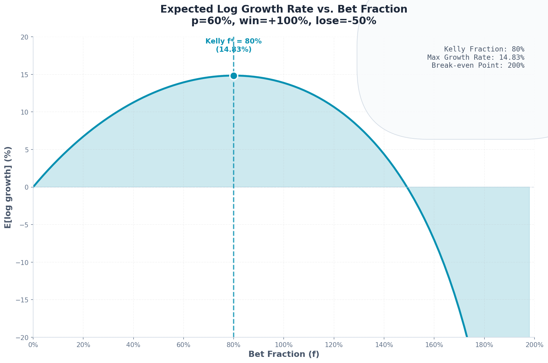
For our coin flip example:

• p = 0.60 (win probability)

• b = 1.00 (win 100% of bet)

• a = 0.50 (lose 50% of bet)

f* = (pb - qa) / (ab)
   = (0.60 × 1.00 - 0.40 × 0.50) / (0.50 × 1.00)
   = (0.60 - 0.20) / 0.50
   = 0.40 / 0.50
   = 0.80

Kelly says: Bet 80% of your bankroll each flip.

Let’s verify this maximizes growth:

f       E[log growth]
---     --------------
0.10    3.67%
0.20    6.87%
0.40    11.51%
0.60    14.51%
0.80    15.22%  ← maximum
1.00    13.86%
1.20    10.40%

Kelly found the peak. Bet more than 80% and your growth rate decreases despite having positive expectation.

This is counterintuitive. Why would betting more reduce growth?

---

4. Why Over-Betting Destroys Wealth

The answer is volatility drag.

Consider two scenarios with the same arithmetic mean:

Scenario A: +50%, +50%

$100 → $150 → $225 (geometric mean: +50%)

Scenario B: +100%, 0%

$100 → $200 → $200 (geometric mean: +41.4%)

Scenario C: +200%, -50%

$100 → $300 → $150 (geometric mean: +22.5%)

All three have 50% arithmetic average return. But the more volatile paths grow slower.

The mathematical relationship:

Geometric Mean ≈ Arithmetic Mean - (Variance / 2)

This is the volatility tax. Larger bets increase variance. At some point, the variance penalty exceeds the benefit from higher expected returns.

Kelly finds exactly where that tradeoff optimizes.

---

5. Kelly as the Growth-Optimal Strategy

Here’s the remarkable theorem Kelly proved:

Theorem: In repeated betting with fixed odds, Kelly betting maximizes the long-run growth rate. Moreover, any other strategy has probability 1 of eventually being overtaken by Kelly.

Proof sketch:

Let W_K(n) be wealth after n bets using Kelly, and W_A(n) using any alternative strategy.

The growth rates are:

g_K = lim(n→∞) (1/n) × ln(W_K(n))
g_A = lim(n→∞) (1/n) × ln(W_A(n))

By the law of large numbers:

g_K = p × ln(1 + f*b) + q × ln(1 - f*a)
g_A = p × ln(1 + fab) + q × ln(1 - faa)

Since f* maximizes the right-hand side, g_K ≥ g_A with equality only when f_A = f*.

For the “probability 1 of overtaking” result:

ln(W_K(n) / W_A(n)) = n × (g_K - g_A) + o(n)

As n → ∞, this diverges to +∞ whenever g_K > g_A.

Translation: Given enough time, Kelly beats everything else. Not in expectation—with probability 1.

---

6. The Kelly Criterion for Continuous Returns

Real markets don’t have discrete win/lose outcomes. Stock returns are continuous.

For a normally distributed return with:

• μ = expected return

• σ = volatility

• r = risk-free rate

The Kelly fraction becomes:

f* = (μ - r) / σ²

This is the continuous Kelly formula. It says your position size should be proportional to:

• Excess return (numerator): Higher alpha → larger position

• Inverse variance (denominator): Higher volatility → smaller position

Example: SPY Allocation

Historical SPY parameters (roughly):

• μ ≈ 10% annual return

• σ ≈ 16% annual volatility

• r ≈ 5% risk-free rate

f* = (0.10 - 0.05) / (0.16)²
   = 0.05 / 0.0256
   = 1.95

Kelly says: 195% allocation to SPY (i.e., 1.95x leverage).

This immediately raises red flags. Levering up 2x to buy the S&P 500? That feels aggressive. We’ll address this in Part 2.

---

7. Kelly vs. Mean-Variance Optimization

The Kelly formula looks suspiciously similar to mean-variance portfolio optimization.

Mean-variance (Markowitz) optimizes:

max E[R] - (λ/2) × Var[R]

where λ is a risk-aversion parameter.

Kelly optimizes:

max E[ln(1 + R)] ≈ max E[R] - (1/2) × Var[R]

The Taylor expansion of log return reveals that Kelly is equivalent to mean-variance with λ = 1.

This means:

• Kelly is more aggressive than most “risk-averse” portfolios

• Kelly is less aggressive than risk-neutral maximizing

• Kelly has a specific, principled reason for its risk tolerance: long-run growth maximization

---

8. The Sharpe Ratio Connection

There’s actually a rather elegant relationship between Kelly and Sharpe ratio.

For normally distributed returns:

f* = (μ - r) / σ² = [(μ - r) / σ] × (1 / σ) = SR / σ

Where SR = Sharpe ratio.

This means:

Expected growth rate = (1/2) × f* × (μ - r) = (1/2) × SR² 

The Kelly growth rate equals half the squared Sharpe ratio.

Implications:

Sharpe Ratio Kelly Growth Rate 0.5 12.5% per year 1.0 50.0% per year 1.5 112.5% per year 2.0 200.0% per year

A Sharpe ratio of 2 (rare for any sustained strategy) implies Kelly-optimal growth of 200% annually. No wonder quants chase Sharpe.

---

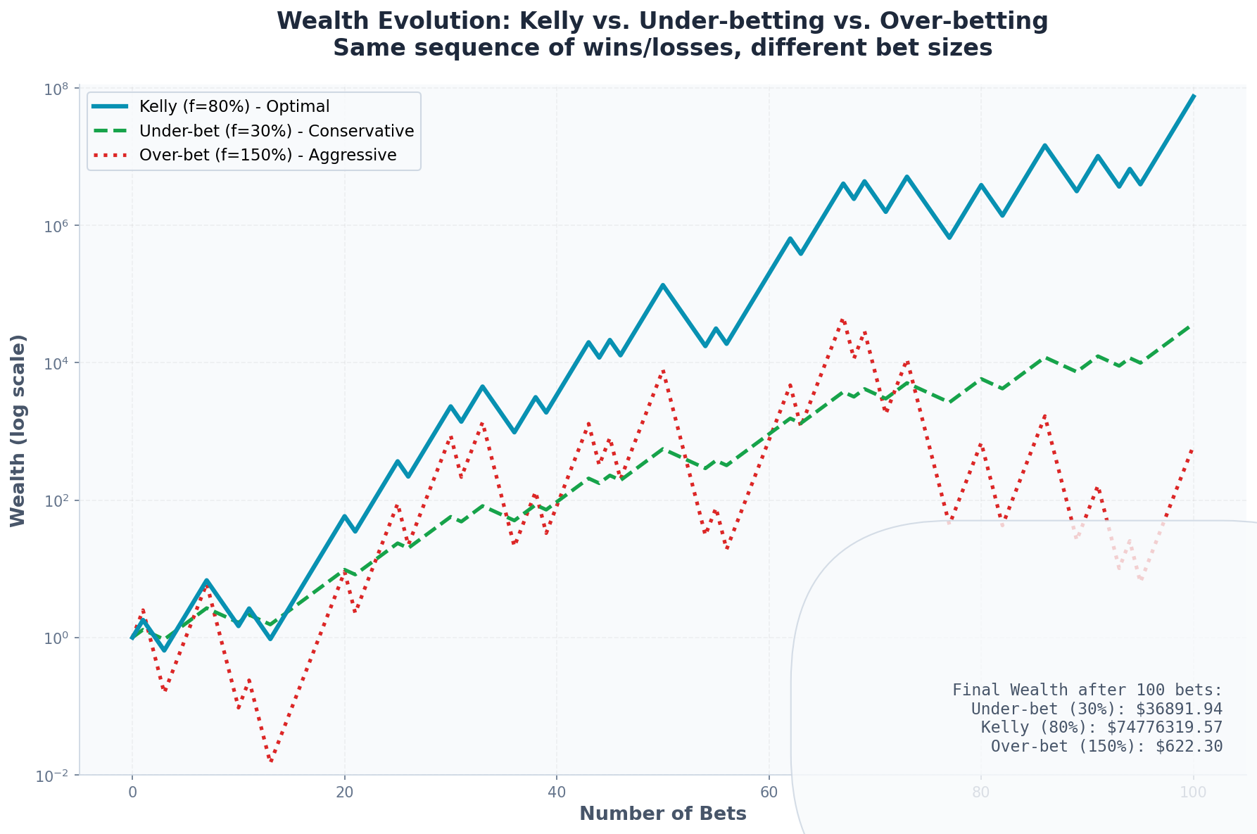
9. Kelly Betting in Practice: A Simulation

Let’s simulate 10,000 paths of 1,000 bets each for our original coin flip game.

Parameters:

• Win probability: 60%

• Win payoff: +100%

• Lose payoff: -50%

• Kelly fraction: 80%

Results at f = 80% (Kelly):

Median final wealth:    $3,142,857 (from $1)
Mean final wealth:      $47,891,203
5th percentile:         $12,847
95th percentile:        $298,471,205
Probability of ruin:    0%

Results at f = 100% (over-betting):

Median final wealth:    $1,024,712
Mean final wealth:      $89,412,847 (higher!)
5th percentile:         $247
95th percentile:        $892,471,028
Probability of ruin:    0%

Results at f = 150% (way over-betting):

Median final wealth:    $0.12
Mean final wealth:      $712,481,920 (even higher!)
5th percentile:         $0.00
95th percentile:        $4,128
Probability of ruin:    78.2%

Notice the paradox: Over-betting increases expected wealth but destroys median wealth.

This is because over-betting creates extreme positive skew. A few paths become astronomically rich, pulling up the mean. But most paths go broke.

Kelly maximizes the median and the geometric mean—what you’ll actually experience on a typical path.

---

10. What Kelly Assumes (And Why It Matters)

The Kelly criterion is optimal given certain assumptions:

1. Known probabilities: You know p and b exactly

2. Repeated bets: The same game plays forever

3. No constraints: You can bet any fraction, including leverage

4. Logarithmic utility: You care about long-run growth

5. Thin tails: Returns are well-behaved (no black swans)

6. Ergodicity: Time averages equal ensemble averages

Every one of these assumptions is violated in real markets.

• We don’t know true probabilities—we estimate them

• Markets change—regimes shift

• Leverage has costs and limits

• Drawdowns hurt beyond log utility

• Fat tails exist

• Single paths can diverge from expectation

Part 2 will explore what happens when these assumptions break.

---

11. Summary: The Kelly Foundation

The Kelly criterion says:

f* = (pb - qa) / ab    (discrete version)
f* = (μ - r) / σ²       (continuous version)
f* = SR / σ             (Sharpe ratio version)

It maximizes long-run growth by balancing expected return against volatility drag.

Key insights:

1. There’s an optimal bet size that’s less than “all-in”

2. Over-betting reduces growth even with positive expectation

3. Kelly is aggressive—often recommending leverage

4. Growth rate scales with Sharpe² / 2—Sharpe matters enormously

5. Kelly beats alternatives with probability 1 over time

But Kelly is also fragile. It assumes you know the parameters perfectly, that the game never changes, and that you can tolerate the drawdowns.

In Part 2, we’ll see exactly how Kelly fails when these assumptions break—and what to do about it.

---

In Part 2: When Kelly Goes Wrong — estimation error, fat tails, and why f = 80% might actually mean f = 20%.*

---

This post is about methodology, not recommendations. The Kelly criterion can suggest leveraged positions that may be inappropriate for most investors. If you find errors in my math, let me know.

The information presented in Math & Markets is not investment or financial advice and should not be construed as such.

---