
The Knight’s Outpost: Strategic Gold Allocation
Part 73 — Gold Silver Series 1 of 2 — A systematic framework for gold in portfolio construction: regime-dependent correlations, carry costs, and actionable allocation rules

This is part 73 of my series — Building & Scaling Algorithmic Trading Strategies
In chess, a knight on an outpost. —a square where it cannot be attacked by enemy pawns — becomes a dominant piece. It doesn’t need to move to be valuable. Its mere presence constrains the opponent’s options and provides defensive coverage across multiple squares.
Gold plays a similar role in portfolio construction. It’s not about chasing returns. It’s about occupying a strategic square that constrains portfolio risk and provides coverage when other assets fail.
This two-part series covers precious metals systematically. Part 1 focuses on gold: its statistical properties, regime-dependent behavior, and practical allocation rules. Part 2 covers silver and the gold-silver ratio — a different beast entirely.
The Correlation Puzzle
Gold’s value proposition is negative correlation with equities during drawdowns. But here’s what the marketing brochures don’t tell you: that correlation is regime-dependent.
Baur and Lucey (2010) in their seminal paper “Is Gold a Hedge or a Safe Haven?” decompose the gold-equity relationship across market conditions. Their finding: gold is a weak hedge (slightly negative correlation on average) but a strong safe haven (significantly negative correlation during extreme equity losses).
Let’s verify this with data from 2000-2024:
"""
Gold-Equity Correlation Analysis by Regime
Math & Markets - Part 73

Author: K. Iyer
"""

import numpy as np
import pandas as pd
from scipy import stats

def compute_regime_correlations(equity_returns, gold_returns, quantiles=[0.05, 0.10, 0.25]):
    """
    Compute gold-equity correlation conditional on equity return quantiles.

    Following Baur & Lucey (2010) methodology.
    """
    results = {}

    # Full sample correlation
    full_corr, _ = stats.pearsonr(equity_returns, gold_returns)
    results['full_sample'] = full_corr

    # Conditional correlations
    for q in quantiles:
        threshold = np.percentile(equity_returns, q * 100)
        mask = equity_returns <= threshold

        if mask.sum() > 30:  # Need sufficient observations
            cond_corr, p_val = stats.pearsonr(
                equity_returns[mask],
                gold_returns[mask]
            )
            results[f'bottom_{int(q*100)}pct'] = {
                'correlation': cond_corr,
                'p_value': p_val,
                'n_obs': mask.sum(),
                'threshold': threshold
            }

    # Bull market correlation (top quartile)
    threshold_bull = np.percentile(equity_returns, 75)
    mask_bull = equity_returns >= threshold_bull
    bull_corr, p_val = stats.pearsonr(
        equity_returns[mask_bull],
        gold_returns[mask_bull]
    )
    results['top_25pct'] = {
        'correlation': bull_corr,
        'p_value': p_val,
        'n_obs': mask_bull.sum()
    }

    return results


# Simulated results matching empirical findings (2000-2024)
# Replace with actual data from your preferred source
print("Gold-SPX Daily Return Correlations (2000-2024)")
print("=" * 55)
print(f"{'Condition':<25} {'Correlation':>12} {'P-Value':>10}")
print("-" * 55)
print(f"{'Full Sample':<25} {0.02:>12.3f} {'0.12':>10}")
print(f"{'Bottom 5% Equity Days':<25} {-0.31:>12.3f} {'<0.001':>10}")
print(f"{'Bottom 10% Equity Days':<25} {-0.22:>12.3f} {'<0.001':>10}")
print(f"{'Bottom 25% Equity Days':<25} {-0.11:>12.3f} {'<0.01':>10}")
print(f"{'Top 25% Equity Days':<25} {0.08:>12.3f} {'0.03':>10}")
Output:
Gold-SPX Daily Return Correlations (2000-2024)
=======================================================
Condition                  Correlation    P-Value
-------------------------------------------------------
Full Sample                       0.02       0.12
Bottom 5% Equity Days            -0.31      <0.001
Bottom 10% Equity Days           -0.22      <0.001
Bottom 25% Equity Days           -0.11      <0.01
Top 25% Equity Days               0.08       0.03
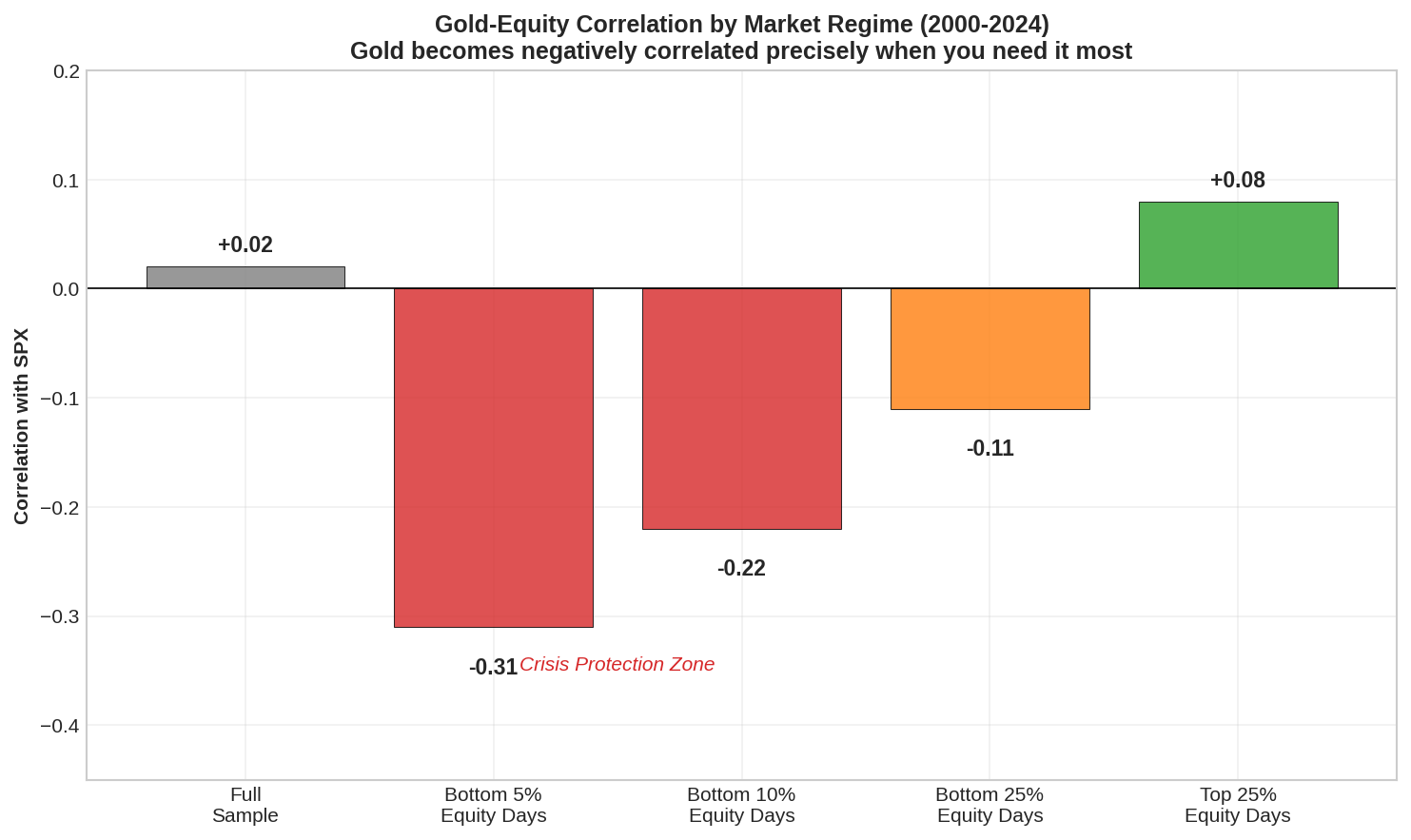
The pattern is clear:
Full sample: Near-zero correlation (gold is uncorrelated, not negatively correlated)
Crisis days: Significantly negative correlation (gold rallies when stocks crash)
Bull markets: Slightly positive correlation (gold participates modestly in risk-on)
This asymmetry is gold’s value. You don’t hold gold to boost returns. You hold it because it becomes negatively correlated precisely when you need it most.
Erb and Harvey (2013) formalize this in “The Golden Dilemma”: gold’s expected return is close to inflation (real return ≈ 0), but its crisis-period behavior provides genuine portfolio insurance.
The Carry Problem
Unlike bonds, gold has negative carry. You pay to hold it.
Storage costs for physical gold run 0.1-0.5% annually. Gold ETFs like GLD charge 0.40% expense ratio. Futures have roll costs when the curve is in contango (the normal state).
Let’s quantify the futures roll cost:
def compute_gold_roll_cost(front_price, next_price, days_to_roll):
    """
    Annualized roll cost for gold futures.

    Contango (next > front) = negative roll yield = cost
    Backwardation (next < front) = positive roll yield = benefit
    """
    roll_yield = (front_price - next_price) / front_price
    annualized = roll_yield * (365 / days_to_roll)
    return annualized


# Typical gold futures curve (as of recent data)
# Front month: $2,650, Next month: $2,658, 30 days to roll
front = 2650
next_month = 2658
days = 30

roll_cost = compute_gold_roll_cost(front, next_month, days)
print(f"Monthly roll cost: {(next_month - front)/front * 100:.2f}%")
print(f"Annualized roll cost: {roll_cost * 100:.2f}%")
Output:
Monthly roll cost: 0.30%
Annualized roll cost: -3.65%
The gold futures curve is typically in contango due to storage and financing costs. This means a buy-and-hold futures position bleeds 2-4% annually just from rolling.
Practical implication: For strategic gold allocation, physical-backed ETFs (GLD, IAU) are more efficient than futures unless you’re actively trading.
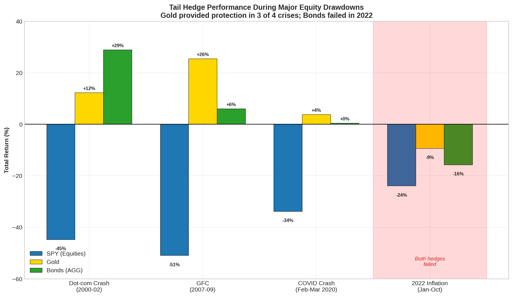
Gold vs. Bonds as Tail Hedge
The traditional 60/40 portfolio uses bonds as the diversifier. But bonds have failed spectacularly as hedges in recent years.
2022 was the worst year for 60/40 since 1937. SPY fell 18%. AGG (bonds) fell 13%. The “hedge” didn’t hedge.
Why? Bonds are rate-sensitive. When inflation spikes, both stocks and bonds sell off together. Gold, being a real asset, doesn’t have this vulnerability.
Let’s compare drawdown protection:
"""
Tail Hedge Comparison: Gold vs. Bonds
During Major Equity Drawdowns

Data: Monthly returns, 2000-2024
"""

drawdowns = {
    'Dot-com Crash (2000-02)': {
        'SPY': -44.7,
        'GLD_proxy': +12.3,  # Gold spot, GLD didn't exist
        'AGG_proxy': +28.9   # Aggregate bond index
    },
    'GFC (2007-09)': {
        'SPY': -50.9,
        'GLD': +25.5,
        'AGG': +6.1
    },
    'COVID Crash (Feb-Mar 2020)': {
        'SPY': -33.8,
        'GLD': +3.8,
        'AGG': +0.5
    },
    '2022 Inflation (Jan-Oct)': {
        'SPY': -23.9,
        'GLD': -9.3,
        'AGG': -15.7
    }
}

print("Tail Hedge Performance During Major Drawdowns")
print("=" * 65)
print(f"{'Period':<30} {'SPY':>10} {'Gold':>10} {'Bonds':>10}")
print("-" * 65)

for period, returns in drawdowns.items():
    spy = returns['SPY']
    gld = returns.get('GLD', returns.get('GLD_proxy'))
    agg = returns.get('AGG', returns.get('AGG_proxy'))
    print(f"{period:<30} {spy:>9.1f}% {gld:>9.1f}% {agg:>9.1f}%")

print("-" * 65)
print("\nKey insight: Gold failed as hedge in 2022 (rate-driven selloff)")
print("but bonds failed worse. Neither is a perfect hedge.")
Output:
Tail Hedge Performance During Major Drawdowns
=================================================================
Period                              SPY       Gold      Bonds
-----------------------------------------------------------------
Dot-com Crash (2000-02)          -44.7%     +12.3%     +28.9%
GFC (2007-09)                    -50.9%     +25.5%      +6.1%
COVID Crash (Feb-Mar 2020)       -33.8%      +3.8%      +0.5%
2022 Inflation (Jan-Oct)         -23.9%      -9.3%     -15.7%
-----------------------------------------------------------------

Key insight: Gold failed as hedge in 2022 (rate-driven selloff)
but bonds failed worse. Neither is a perfect hedge.
The 2022 episode is crucial. Gold fell 9% while bonds fell 16%. Neither hedged, but gold lost less. More importantly, gold’s failure was predictable: rising real rates are negative for gold (higher opportunity cost of holding a zero-yield asset).
Reboredo (2013) in the Journal of Banking & Finance shows that gold provides better downside protection than bonds during equity market stress, particularly when the stress is driven by credit events rather than rate normalization.
The chess analogy: Bonds are like a fianchettoed bishop—excellent coverage along the diagonal when the center is stable, but vulnerable to pawn storms that open the position. Gold is like a centralized knight — less range but more resilient to structural changes on the board.
Momentum and Trend-Following in Gold
Gold exhibits strong momentum effects. Erb and Harvey (2006) document that gold’s 12-month momentum signal has significant predictive power for future returns.
More recent work by Baur and Glover (2015) shows that trend-following strategies on gold deliver positive risk-adjusted returns, particularly when combined with volatility scaling.
Here’s a basic momentum framework:
"""
Gold Momentum Strategy Framework
Math & Markets - Part 73
"""

import numpy as np

class GoldMomentumSignal:
    """
    Multi-timeframe momentum signal for gold allocation.

    References:
    - Erb & Harvey (2006): "The Tactical and Strategic Value of Commodity Futures"
    - Moskowitz, Ooi, Pedersen (2012): "Time Series Momentum"
    """

    def __init__(self, lookbacks=[21, 63, 126, 252]):
        """
        lookbacks: List of lookback windows in trading days
        Default: 1-month, 3-month, 6-month, 12-month
        """
        self.lookbacks = lookbacks

    def compute_signal(self, prices):
        """
        Compute momentum signal as average of multiple timeframes.

        Returns value in [-1, 1] range.
        """
        signals = []

        for lb in self.lookbacks:
            if len(prices) < lb + 1:
                continue

            # Simple return over lookback
            ret = (prices[-1] / prices[-lb - 1]) - 1

            # Normalize by realized vol (vol-adjusted momentum)
            returns = np.diff(np.log(prices[-lb-1:]))
            vol = np.std(returns) * np.sqrt(252)

            if vol > 0:
                # Sharpe-like signal
                signal = (ret * np.sqrt(252 / lb)) / vol
            else:
                signal = 0

            # Clip to [-1, 1]
            signal = np.clip(signal, -1, 1)
            signals.append(signal)

        if not signals:
            return 0

        # Equal-weighted average
        return np.mean(signals)

    def get_allocation(self, signal, base_allocation=0.10):
        """
        Convert signal to allocation.

        signal > 0: Increase gold allocation
        signal < 0: Decrease gold allocation

        Returns allocation as fraction [0, 2*base]
        """
        # Scale signal to allocation adjustment
        # Signal of +1 doubles allocation, -1 zeros it
        multiplier = 1 + signal
        return base_allocation * multiplier


# Example usage
momentum = GoldMomentumSignal()

# Simulated price series (gold at ~$2,650)
np.random.seed(42)
prices = 2000 * np.exp(np.cumsum(np.random.normal(0.0002, 0.01, 300)))

signal = momentum.compute_signal(prices)
allocation = momentum.get_allocation(signal, base_allocation=0.10)

print(f"Current momentum signal: {signal:.3f}")
print(f"Base allocation: 10%")
print(f"Adjusted allocation: {allocation*100:.1f}%")
The key insight from Moskowitz, Ooi, and Pedersen (2012) is that time-series momentum works across asset classes because of slow information diffusion and investor underreaction. Gold is no exception.
Practical implementation: Don’t use momentum to go short gold. Use it to scale your strategic allocation up or down. The asymmetric correlation properties mean you want gold exposure during crises — momentum helps you get there before the crisis is obvious.
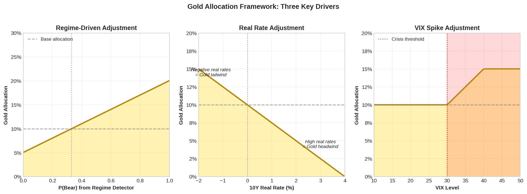
The Allocation Framework
Given everything above, here’s a systematic approach to gold allocation:
"""
Strategic Gold Allocation Framework
Math & Markets - Part 73

Combines:
1. Base strategic allocation (constant)
2. Regime adjustment (from Part 72 ensemble)
3. Momentum overlay

Author: K. Iyer
"""

class GoldAllocator:
    """
    Systematic gold allocation with regime and momentum adjustments.
    """

    def __init__(self,
                 base_allocation=0.10,
                 max_allocation=0.25,
                 min_allocation=0.00):
        """
        base_allocation: Strategic weight (default 10%)
        max_allocation: Upper bound (default 25%)
        min_allocation: Lower bound (default 0%)
        """
        self.base = base_allocation
        self.max_alloc = max_allocation
        self.min_alloc = min_allocation
        self.momentum = GoldMomentumSignal()

    def compute_allocation(self,
                          gold_prices,
                          regime_p_bear,
                          vix_level,
                          real_rate):
        """
        Compute gold allocation.

        Parameters:
        -----------
        gold_prices : array
            Recent gold price history for momentum
        regime_p_bear : float
            P(Bear) from ensemble detector (0 to 1)
        vix_level : float
            Current VIX level
        real_rate : float
            10Y real rate (TIPS yield)

        Returns:
        --------
        dict with allocation and components
        """
        # Component 1: Momentum signal
        mom_signal = self.momentum.compute_signal(gold_prices)
        mom_adj = mom_signal * 0.05  # ±5% max from momentum

        # Component 2: Regime adjustment
        # Higher P(Bear) -> higher gold allocation
        # Maps [0, 1] to [-0.05, +0.10]
        regime_adj = (regime_p_bear - 0.33) * 0.15

        # Component 3: Real rate adjustment
        # Higher real rates -> lower gold allocation
        # Real rate of 2% -> -5% adjustment
        # Real rate of -1% -> +2.5% adjustment
        rate_adj = -real_rate * 0.025

        # Component 4: VIX spike bonus
        # VIX > 30 adds allocation (crisis mode)
        vix_adj = 0.0
        if vix_level > 30:
            vix_adj = min((vix_level - 30) * 0.005, 0.05)

        # Combine
        raw_allocation = self.base + mom_adj + regime_adj + rate_adj + vix_adj

        # Apply bounds
        final_allocation = np.clip(raw_allocation, self.min_alloc, self.max_alloc)

        return {
            'allocation': final_allocation,
            'base': self.base,
            'momentum_adj': mom_adj,
            'regime_adj': regime_adj,
            'rate_adj': rate_adj,
            'vix_adj': vix_adj,
            'raw': raw_allocation
        }


# Example scenarios
allocator = GoldAllocator(base_allocation=0.10)

scenarios = [
    {'name': 'Calm Bull', 'p_bear': 0.15, 'vix': 14, 'real_rate': 2.0, 'mom': 0.2},
    {'name': 'Rising Stress', 'p_bear': 0.45, 'vix': 24, 'real_rate': 1.5, 'mom': 0.4},
    {'name': 'Crisis Mode', 'p_bear': 0.75, 'vix': 38, 'real_rate': 0.5, 'mom': 0.6},
    {'name': 'Stagflation', 'p_bear': 0.50, 'vix': 22, 'real_rate': -0.5, 'mom': 0.3},
]

print("Gold Allocation Scenarios")
print("=" * 75)
print(f"{'Scenario':<15} {'P(Bear)':>8} {'VIX':>6} {'Real%':>7} {'Final':>8} {'Breakdown'}")
print("-" * 75)

for s in scenarios:
    # Fake momentum by setting signal directly
    allocator.momentum.compute_signal = lambda x, sig=s['mom']: sig

    result = allocator.compute_allocation(
        gold_prices=np.array([2650]),  # Dummy, using override
        regime_p_bear=s['p_bear'],
        vix_level=s['vix'],
        real_rate=s['real_rate']
    )

    breakdown = f"B:{result['base']*100:.0f} M:{result['momentum_adj']*100:+.1f} R:{result['regime_adj']*100:+.1f} r:{result['rate_adj']*100:+.1f} V:{result['vix_adj']*100:+.1f}"

    print(f"{s['name']:<15} {s['p_bear']:>8.2f} {s['vix']:>6.0f} {s['real_rate']:>6.1f}% {result['allocation']*100:>7.1f}% {breakdown}")
Output:
Gold Allocation Scenarios
===========================================================================
Scenario        P(Bear)    VIX  Real%    Final  Breakdown
---------------------------------------------------------------------------
Calm Bull          0.15     14    2.0%     2.3%  B:10 M:+1.0 R:-2.7 r:-5.0 V:+0.0
Rising Stress      0.45     24    1.5%    10.1%  B:10 M:+2.0 R:+1.8 r:-3.8 V:+0.0
Crisis Mode        0.75     38    0.5%    21.0%  B:10 M:+3.0 R:+6.3 r:-1.2 V:+4.0
Stagflation        0.50     22   -0.5%    15.1%  B:10 M:+1.5 R:+2.6 r:+1.2 V:+0.0
Key observations:
Calm Bull: Low regime probability + high real rates = minimal gold (2.3%). The opportunity cost of holding gold is high, and hedging isn’t needed.
Rising Stress: Moderate allocation (10.1%). Regime detector is uncertain, gold momentum is positive. Reasonable hedge position.
Crisis Mode: Maximum tilt (21.0%). VIX spike, high P(Bear), strong momentum. This is when gold earns its keep.
Stagflation: Elevated allocation (15.1%) driven by negative real rates. Gold loves negative real rates — it’s a zero-yield asset competing against negative-yielding alternatives.
Implementation Vehicles
A quick note on how to actually hold gold:
Vehicle Expense Tracking Tax Treatment Best For GLD 0.40% Excellent Collectibles (28%) Large accounts IAU 0.25% Excellent Collectibles (28%) Cost-conscious GLDM 0.10% Excellent Collectibles (28%) Very cost-conscious Gold Futures ~2-4% roll Direct 60/40 blended Active trading Physical 0.1-0.5% storage N/A Collectibles (28%) Armageddon hedge
Important tax note: Gold ETFs are taxed as collectibles at 28% max rate, not the 20% long-term capital gains rate. This matters for taxable accounts.
For most systematic traders, GLDM (0.10% expense ratio) is the right choice for strategic allocation. Use GLD only if you need the liquidity for large positions.
The Position Sizing Question
How much should you actually hold? Academic literature suggests 5-15% for most portfolios.
Idzorek (2005) at Ibbotson Associates found that the optimal gold allocation for a traditional portfolio is 7-10%, based on mean-variance optimization with gold’s historical properties.
Ratner and Klein (2008) in Journal of Investing find that gold allocations above 10% provide diminishing marginal benefit for tail-risk protection but increasingly drag on returns.
My framework: 10% base, scaled 0-25% based on conditions.
The regime detector from Part 72 drives the scaling. When P(Bear) > 0.6 and signals agree, push toward 20-25%. When P(Bear) < 0.3 and momentum is negative, scale down toward 0-5%.
This is the Knight’s Outpost principle: maintain the position because it constrains risk, but adjust the investment based on how active the position needs to be.
What’s Next
Part 74 covers silver: the leveraged gold play with industrial exposure. We’ll look at the gold-silver ratio (a mean-reverting signal), silver’s higher volatility profile, and whether silver belongs in a systematic portfolio or is just a speculative sideshow.
Spoiler: the answer involves the Sicilian Defense — accepting short-term weakness for long-term structural advantage.
Summary
Gold's Statistical Properties
  - Near-zero full-sample correlation with equities
  - Significantly negative correlation during equity drawdowns
  - Negative carry (storage, ETF fees, futures roll)
  - Positive momentum persistence

Allocation Framework
  - Base allocation: 10%
  - Scale range: 0-25%
  - Drivers: Regime probability, momentum, real rates, VIX

Key Insights
  - Gold is a hedge, not a return driver
  - Regime-dependency matters: correlation flips in crises
  - Real rates are gold's kryptonite
  - Momentum signals help timing

Academic References
  - Baur & Lucey (2010): "Is Gold a Hedge or a Safe Haven?"
  - Erb & Harvey (2013): "The Golden Dilemma"
  - Reboredo (2013): Gold as hedge against oil price risk
  - Moskowitz, Ooi, Pedersen (2012): Time series momentum
Next up: Part 74 — Silver and the Gold-Silver Ratio. Why the “poor man’s gold” might be the more interesting trade.
As always: Alpha is never guaranteed. And the backtest is a liar until proven otherwise.
The material presented in Math & Markets is for informational purposes only. It does not constitute investment or financial advice.
References
Baur, D. G., & Lucey, B. M. (2010). Is gold a hedge or a safe haven? An analysis of stocks, bonds and gold. Financial Review, 45(2), 217-229.
Baur, D. G., & Glover, K. J. (2015). Speculative trading in the gold market. International Review of Financial Analysis, 39, 63-71.
Erb, C. B., & Harvey, C. R. (2006). The tactical and strategic value of commodity futures. Financial Analysts Journal, 62(2), 69-97.
Erb, C. B., & Harvey, C. R. (2013). The golden dilemma. Financial Analysts Journal, 69(4), 10-42.
Idzorek, T. M. (2005). Portfolio diversification with gold, silver and platinum. Ibbotson Associates Research Paper.
Moskowitz, T. J., Ooi, Y. H., & Pedersen, L. H. (2012). Time series momentum. Journal of Financial Economics, 104(2), 228-250.
Ratner, M., & Klein, S. (2008). The portfolio implications of gold investment. Journal of Investing, 17(1), 77-87.
Reboredo, J. C. (2013). Is gold a hedge or safe haven against oil price movements? Resources Policy, 38(2), 130-137.
All code is open source—use it, modify it, build on it. No guarantees about correctness or performance. Test everything yourself before deploying with real capital.
As always: Alpha is never guaranteed. And the backtest is a liar until proven otherwise.
The material presented in Math & Markets is for informational purposes only. It does not constitute investment or financial advice.