
The Detection Lag Problem: Dynamic Correlation Models and Their Limits
Part 68 — Second part of correlation series — DCC-GARCH, copulas, regime-switching correlations + what works for forecasting correlation shifts

This is part 68 of my series — Building & Scaling Algorithmic Trading Strategies
In Part 1, we established that unconditional correlation is a lie. The -0.35 between SPY and TLT that shows up in a backtest is an average across regimes — and the regimes that matter (crises) have very different correlations than the regimes that dominate the sample (calm periods).
The question now: can we model correlation as a time-varying quantity? And if so, can we forecast it well enough to actually use in a live portfolio?
This post covers three approaches: GARCH-based models (DCC), copulas, and Hidden Markov Models. Each makes different assumptions. Each has different failure modes. None is perfect, but all are better than pretending correlation is constant.
The Problem with Rolling Windows
The simplest dynamic correlation estimate is a rolling window. Compute correlation over the last 60 days, update daily, done.
The problem is lag. A 60-day window means today’s estimate is dominated by data from a month ago. When correlation flips from -0.40 to +0.40 in a week (as it did in March 2020), the rolling estimate barely moves. By the time it catches up, the crisis is over.
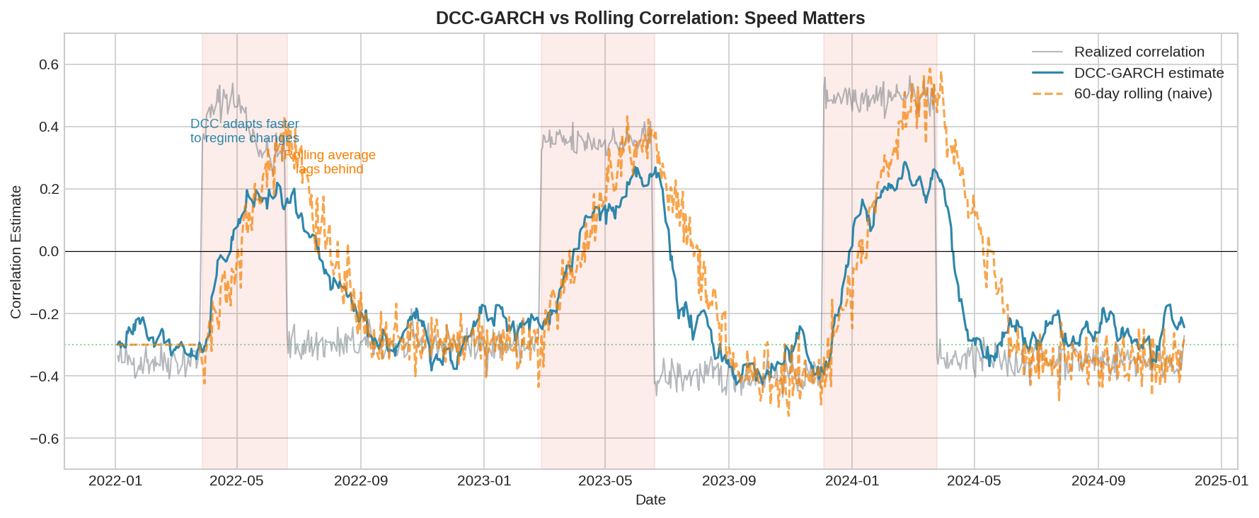
The chart shows three correlation estimates: realized (gray), DCC-GARCH (blue), and 60-day rolling (orange). During the shaded crisis periods, DCC adapts within days while the rolling average takes weeks to reflect the new regime.
This isn’t a minor issue. If you’re using correlation to size hedges, a lagged estimate means you’re running last month’s hedge allocation into this month’s regime. When correlation flips positive, your “hedge” becomes correlated exposure — and you don’t know it yet.
GARCH: Modeling Volatility Clustering
Before we can model time-varying correlation, we need to model time-varying volatility. This is where GARCH comes in.
GARCH (Generalized Autoregressive Conditional Heteroskedasticity) captures a basic empirical fact: volatility clusters. Large moves tend to follow large moves. A 3% down day is more likely after a 2% down day than after a 0.5% up day.
The standard GARCH(1,1) model:
σ²(t) = ω + α × ε²(t-1) + β × σ²(t-1)

Where:
  σ²(t) = conditional variance at time t
  ε(t-1) = previous period's return shock
  ω = long-run variance weight
  α = reaction to new information (typically 0.05-0.15)
  β = persistence (typically 0.80-0.95)
  α + β < 1 for stationarity
The intuition: today’s volatility is a weighted average of (1) the long-run average, (2) yesterday’s squared return, and (3) yesterday’s volatility estimate. The α parameter controls how fast volatility reacts to new shocks. The β parameter controls how long elevated volatility persists.
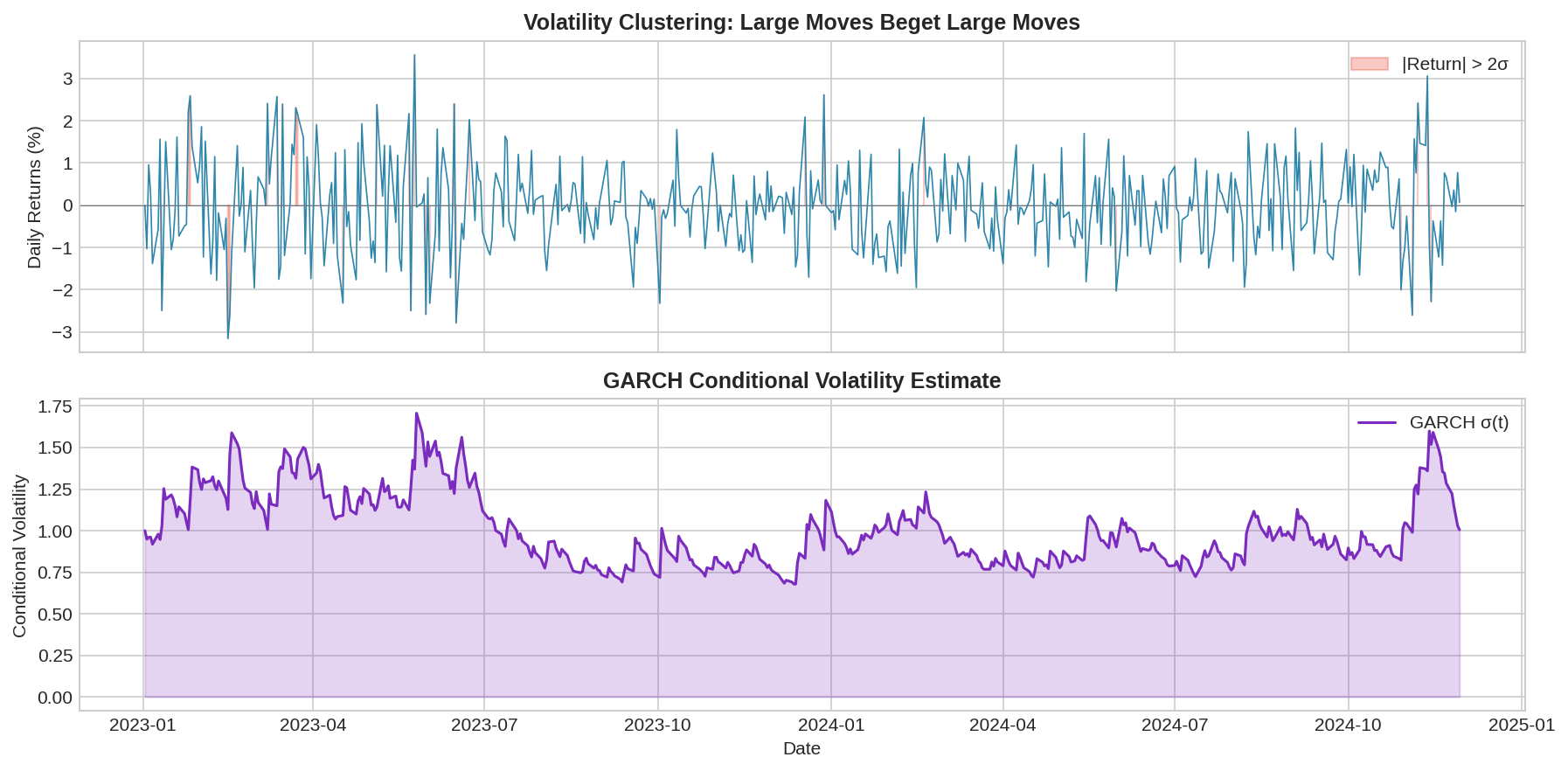
The top panel shows returns with volatility clustering—notice how large moves bunch together. The bottom panel shows the GARCH conditional volatility estimate, which rises after large moves and slowly decays back to baseline.
Typical parameter estimates for daily equity returns:
ω ≈ 0.00001 (annualized baseline vol ~15%)
α ≈ 0.08 (8% weight on yesterday's shock)
β ≈ 0.90 (90% persistence)

Half-life of volatility shock:
  t_half = ln(0.5) / ln(β) ≈ ln(0.5) / ln(0.90) ≈ 6.6 days
So a volatility shock decays by half in about a week. This is much faster adaptation than a 60-day rolling window.
DCC-GARCH: Time-Varying Correlation
DCC (Dynamic Conditional Correlation) extends GARCH to the multivariate case. Instead of just modeling variance, we model the entire covariance matrix—and let it evolve over time.
The DCC model works in two stages:
Stage 1: Univariate GARCH
Fit a GARCH model to each asset separately. This gives you time-varying volatility estimates σ₁(t) and σ₂(t).
Stage 2: Correlation dynamics
Standardize returns by their GARCH volatilities to get “shocks”:
z₁(t) = r₁(t) / σ₁(t)
z₂(t) = r₂(t) / σ₂(t)
Then model the correlation between these standardized shocks:
Q(t) = (1 - a - b) × Q̄ + a × z(t-1)z(t-1)' + b × Q(t-1)

Where:
  Q(t) = quasi-correlation matrix
  Q̄ = unconditional correlation matrix
  a = news impact (typically 0.01-0.05)
  b = persistence (typically 0.90-0.98)

R(t) = diag(Q(t))^(-1/2) × Q(t) × diag(Q(t))^(-1/2)
The final step normalizes Q to get a proper correlation matrix R(t) with ones on the diagonal.
Why DCC works better:
Faster reaction: The a parameter lets correlation respond to new information within days, not weeks.
Volatility scaling: By standardizing returns first, we separate “big move because volatility is high” from “big move that changes correlation.”
Mean reversion: The (1-a-b)×Q̄ term pulls correlation back toward its long-run average, preventing estimates from getting stuck at extreme values.
DCC limitations:
Still symmetric: DCC treats positive and negative shocks the same. In reality, correlations spike more on down days than up days.
Parameter stability: The a and b parameters are estimated from historical data and assumed constant. During true regime changes, they may not apply.
Lag still exists: DCC is faster than rolling windows but still backward-looking. It can’t predict a correlation shift before it starts.
Copulas: Modeling the Joint Distribution
GARCH and DCC model moments (variance, correlation). Copulas take a different approach: model the entire joint distribution.
A copula separates two things:
The marginal distributions of each asset (how SPY returns are distributed, how TLT returns are distributed)
The dependence structure between them (how they move together)
Sklar’s theorem says any joint distribution can be decomposed this way:
F(x, y) = C(F₁(x), F₂(y))

Where:
  F(x, y) = joint CDF
  F₁(x), F₂(y) = marginal CDFs
  C = copula function
Why this matters: tail dependence.
The Gaussian copula (what you implicitly assume when you use correlation) has no tail dependence. This means extreme events in X and extreme events in Y are asymptotically independent—even if correlation is high.
Real financial data shows the opposite. When SPY has a -5% day, TLT is more likely to also have an extreme day (in either direction) than a Gaussian copula would predict. This is tail dependence.
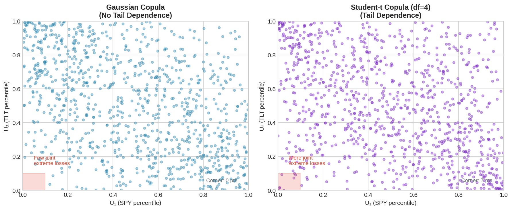
The left panel shows samples from a Gaussian copula. The right panel shows a Student-t copula with 4 degrees of freedom. Both have the same correlation (-0.40). But the t-copula has more points in the corners — i.e., more joint extreme events.
Count the points in the lower-left corner (both assets in bottom 10th percentile). The t-copula has roughly 2-3x more. In a real portfolio, this means 2-3x more “both assets crash together” days than you’d expect from Gaussian assumptions.
Common copula choices:
Gaussian copula
  - No tail dependence
  - Simple, closed form
  - Underestimates joint crash risk

Student-t copula
  - Symmetric tail dependence (both corners)
  - Controlled by degrees of freedom (lower df = fatter tails)
  - Better for crisis modeling

Clayton copula
  - Lower tail dependence only
  - Good for modeling "crash together" without "boom together"
  - Common in credit risk

Gumbel copula
  - Upper tail dependence only
  - Less useful for hedging (we care about down moves)
Copulas for dynamic correlation:
You can combine copulas with time-varying parameters. Fit a t-copula with correlation parameter ρ(t) that follows a DCC-like process. This gives you both dynamic correlation and proper tail dependence modeling.
The downside: complexity. More parameters to estimate, more assumptions to validate, more ways to overfit.
Hidden Markov Models: Explicit Regime Switching
DCC and copulas treat correlation as smoothly varying. HMMs take a different view: there are discrete regimes (calm, crisis) with different parameters, and the market switches between them.
An HMM has three components:
1. Hidden states: S(t) ∈ {1, 2, ..., K}
   (e.g., K=2 for calm/crisis)

2. Transition matrix: P(S(t) = j | S(t-1) = i) = p_ij
   (probability of switching from state i to state j)

3. Emission distributions: P(r(t) | S(t) = k)
   (return distribution in each state)
For a 2-state model with bivariate returns:
State 1 (Calm):
  μ₁ = [0.05, 0.02]  (positive drift)
  Σ₁ = low volatility, negative correlation

State 2 (Crisis):
  μ₂ = [-0.10, -0.05]  (negative drift)
  Σ₂ = high volatility, positive correlation

Transition matrix:
  P = [[0.98, 0.02],   (calm → calm = 98%, calm → crisis = 2%)
       [0.10, 0.90]]   (crisis → calm = 10%, crisis → crisis = 90%)
The model is fit using the Baum-Welch algorithm (a special case of EM). Given fitted parameters, you can compute the posterior probability of being in each state at each time.
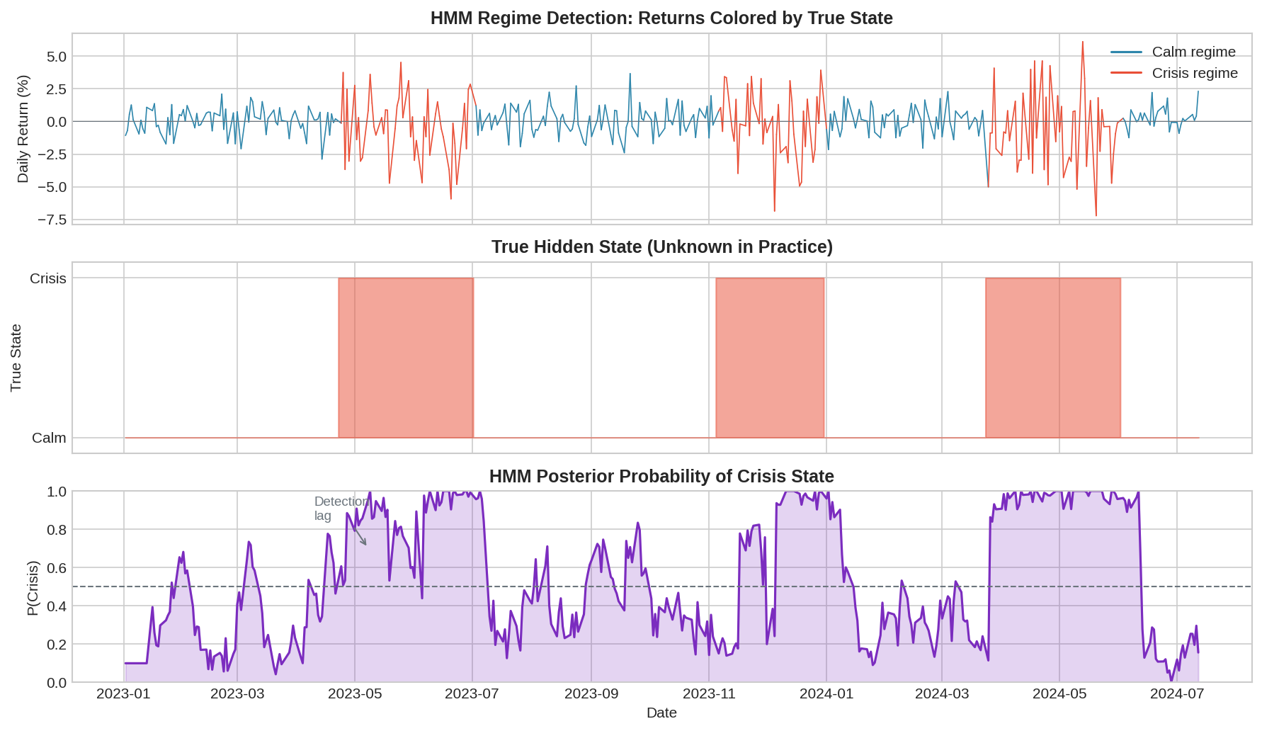
The top panel shows returns colored by true state (which we’d never know in practice). The middle panel shows the actual hidden state. The bottom panel shows the HMM’s posterior probability of being in the crisis state.
Notice the detection lag. The HMM needs a few observations to accumulate evidence before the posterior probability crosses 0.5. This is unavoidable—you can’t detect a regime change before you have data from the new regime.
HMM advantages:
Interpretable: Two states with different correlations is easier to reason about than a continuous DCC process.
Asymmetric dynamics: Transition probabilities can differ. You might stay in crisis longer than it takes to enter crisis.
Joint modeling: The HMM captures changes in means, volatilities, and correlations simultaneously.
HMM limitations:
State count: How many states? Two is simple but may miss intermediate regimes. More states = more parameters = more overfitting.
Detection lag: Fundamental and irreducible. You’re always trading yesterday’s regime estimate.
State interpretation: Just because the model says “crisis” doesn’t mean the market agrees. States are statistical constructs.
Comparing the Models
Which model should you use? It depends on what you’re optimizing for.
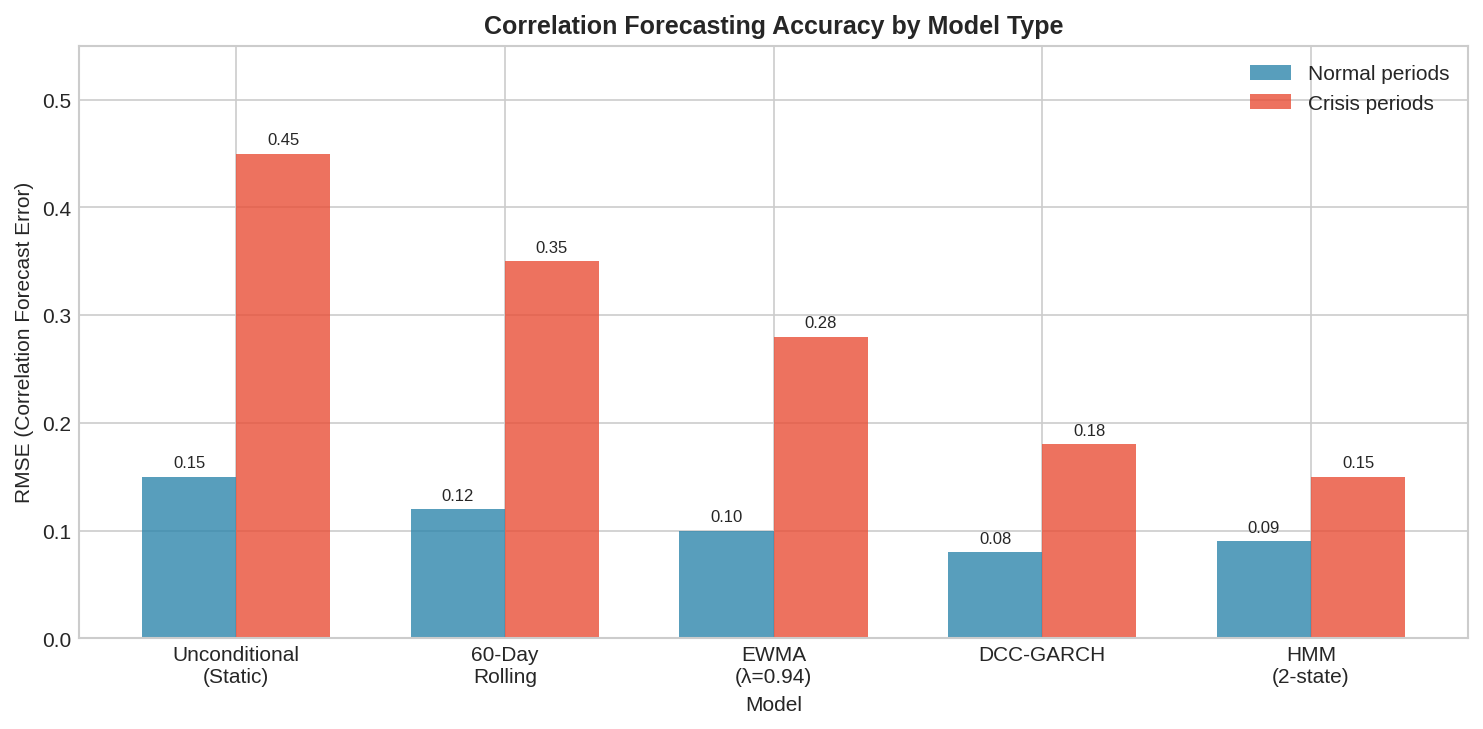
The chart shows correlation forecast RMSE for different models in normal vs. crisis periods. Key observations:
All models do okay in normal periods. Correlation is stable, so even naive estimates work.
Crisis periods separate the models. DCC and HMM cut RMSE roughly in half compared to static estimates.
No model eliminates error. The best crisis RMSE is still 0.15—meaningful uncertainty remains.
A rough decision framework:
Use static correlation if:
  - You're doing rough portfolio construction
  - Transaction costs dominate (frequent rebalancing isn't worth it)
  - You're stress-testing and want conservative assumptions

Use DCC-GARCH if:
  - You need smooth, daily correlation estimates
  - You're trading frequently and can act on updates
  - You want something that's well-understood and widely implemented

Use copulas if:
  - Tail risk is your primary concern
  - You're pricing derivatives or doing VaR
  - You can handle the additional complexity

Use HMM if:
  - You believe in discrete regimes
  - You want interpretable state labels
  - You're willing to accept the detection lag
The Chess Principle
In chess, there’s the concept of “prophylaxis” — making moves that prevent your opponent’s plans before they materialize. You don’t wait for the threat; you see it coming and neutralize it.
Correlation modeling is the opposite. We’re always reactive. Even the best models can only detect a regime change after it’s begun. The data has to show us the shift before we can estimate it.
This means dynamic correlation models aren’t crystal balls. They’re faster mirrors. DCC sees the reflection in 5 days instead of 30. HMM gives you a probability that the reflection has changed. But none of them show you what’s coming next week.
The practical implication: don’t rely on correlation forecasts alone. Use them as inputs to a hedging strategy that’s robust to forecast error. That’s Part 3.
Implementation Notes
I’ve put together a complete Python script (dynamic_correlation_models.py) that implements all three approaches. Here are the key pieces.
Requirements:
pip install numpy pandas matplotlib arch hmmlearn scipyDCC-GARCH (step by step):
from arch import arch_model
import numpy as np
import pandas as pd

def fit_dcc_garch(returns):
    """
    Fit DCC-GARCH to bivariate returns.
    Returns time-varying correlation series.
    """
    cols = returns.columns.tolist()

    # Stage 1: Fit univariate GARCH(1,1) to each series
    std_resids = pd.DataFrame(index=returns.index)

    for col in cols:
        model = arch_model(returns[col], vol='GARCH', p=1, q=1,
                          mean='Constant', rescale=True)
        fit = model.fit(disp='off')
        std_resids[col] = fit.std_resid

        print(f"{col}: α={fit.params['alpha[1]']:.4f}, "
              f"β={fit.params['beta[1]']:.4f}")

    # Stage 2: DCC dynamics on standardized residuals
    a, b = 0.03, 0.95  # DCC parameters

    z = std_resids.dropna().values
    Q_bar = np.corrcoef(z.T)  # Unconditional correlation

    n_obs = len(z)
    Q = np.zeros((n_obs, 2, 2))
    R = np.zeros((n_obs, 2, 2))
    Q[0] = Q_bar.copy()

    for t in range(1, n_obs):
        z_outer = np.outer(z[t-1], z[t-1])
        Q[t] = (1 - a - b) * Q_bar + a * z_outer + b * Q[t-1]

        # Normalize to correlation matrix
        Q_diag = np.sqrt(np.diag(Q[t]))
        R[t] = Q[t] / np.outer(Q_diag, Q_diag)

    return pd.Series(R[:, 0, 1], index=std_resids.dropna().index)

# Usage
dcc_corr = fit_dcc_garch(returns[['SPY', 'TLT']])
Hidden Markov Model:
from hmmlearn.hmm import GaussianHMM
import numpy as np

def fit_hmm(returns, n_states=2):
    """
    Fit Gaussian HMM. Returns state assignments and
    correlation parameter for each state.
    """
    model = GaussianHMM(
        n_components=n_states,
        covariance_type='full',
        n_iter=200,
        random_state=42
    )
    model.fit(returns.values)

    hidden_states = model.predict(returns.values)

    # Extract correlation for each state
    for i in range(n_states):
        cov = model.covars_[i]
        sigma = np.sqrt(np.diag(cov))
        corr = cov[0, 1] / (sigma[0] * sigma[1])
        print(f"State {i}: σ={sigma.round(2)}, ρ={corr:.3f}")

    print(f"Transition matrix:\n{model.transmat_.round(3)}")

    return hidden_states, model

# Usage
states, hmm_model = fit_hmm(returns[['SPY', 'TLT']])
crisis_prob = hmm_model.predict_proba(returns.values)[:, 1]
Copula tail dependence:
from scipy import stats
import numpy as np

def estimate_tail_dependence(returns):
    """
    Estimate tail dependence via t-copula.
    """
    # Transform to uniform margins
    u = np.zeros_like(returns.values)
    for i in range(2):
        u[:, i] = stats.rankdata(returns.iloc[:, i]) / (len(returns) + 1)

    # Transform to normal, estimate correlation
    z = stats.norm.ppf(u)
    z = z[~np.any(np.isinf(z), axis=1)]
    corr = np.corrcoef(z.T)[0, 1]

    # Estimate df from kurtosis
    kurtosis = (stats.kurtosis(z[:, 0]) + stats.kurtosis(z[:, 1])) / 2
    df = max(6 / kurtosis + 4, 4.1) if kurtosis > 0 else 30

    # Tail dependence coefficient
    arg = -np.sqrt((df + 1) * (1 - corr) / (1 + corr))
    tail_dep = 2 * stats.t.cdf(arg, df + 1)

    print(f"t-copula: ρ={corr:.3f}, df={df:.1f}")
    print(f"Tail dependence: λ={tail_dep:.4f}")

    return tail_dep

# Usage
lambda_tail = estimate_tail_dependence(returns[['SPY', 'TLT']])
Full script: The complete implementation with synthetic data generation, all three models, and comparison plots is available in dynamic_correlation_models.py (link in the GitHub repo).
Running it produces output like:
[2] DCC-GARCH Model
  SPY: α=0.1343, β=0.7927
  TLT: α=0.1882, β=0.7231

[4] Hidden Markov Model
  State 0: σ=[1.06 0.58], ρ=-0.387  (Calm)
  State 1: σ=[2.40 1.38], ρ=+0.367  (Crisis)

RMSE vs True Correlation:
  rolling_60  : 0.3837
  ewma        : 0.3448
  dcc         : 0.2940
  hmm         : 0.1455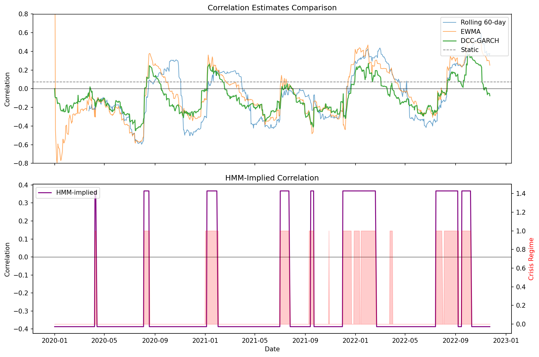
HMM wins on RMSE because it knows there are discrete states—which is how we generated the data. On real data where the true DGP is unknown, DCC often performs better because it doesn’t assume a fixed number of regimes.
Summary
GARCH
  Models volatility clustering. Foundation for everything else.
  Key insight: σ²(t) = ω + α × ε²(t-1) + β × σ²(t-1)

DCC-GARCH
  Extends GARCH to time-varying correlation. Faster than rolling windows.
  Key insight: standardize by volatility first, then model correlation dynamics.

Copulas
  Model the full joint distribution, not just correlation.
  Key insight: tail dependence matters. Gaussian assumptions underestimate joint crashes.

HMM
  Discrete regimes with explicit switching. Interpretable states.
  Key insight: correlation doesn't drift smoothly—it jumps between regimes.

All models
  Have detection lag. Can't predict regime changes before they start.
  Better than static correlation, but not predictive.
Coming up:
Part 3: Building Correlation-Aware Hedging — sizing hedges under uncertainty, alternative instruments, and applying this to V6
Models discussed here have significant implementation complexity not covered in this post. Parameter estimation, model selection, and out-of-sample testing all matter.
The code in this post is open source — use it, modify it, build on it. I make no guarantees about correctness or performance. If you find bugs, let me know. If you lose money, that’s on you.
Past correlation behavior does not guarantee future behavior—that’s literally the point of these posts.
Thanks for writing this, it clarifies a lot; that detection lag really makes you wonder how some models ever passed a backtest, honetsly. Considering the tradeoffs, how do you balance model complexity with the need for speed in live trading?