
Testing the Forecast-to-Fill Model on Gold Futures (arXiv 2511.08571)
Part 25 below is my failed attempt to test the forecast to fill model on limited data

This is part 25 of my series — Building & Scaling Algorithmic Trading Strategies
You don’t always hit home runs. But that’s okay.
Sometimes I see something interesting and I want to “fast and furious” mode to see if it has potential. This is one of those times.
I wanted to see whether the “Forecast-to-Fill” framework from this paper (https://arxiv.org/abs/2511.08571) could be reproduced cleanly inside my research stack — and more importantly, whether it produces meaningful out-of-sample results on something simple like gold futures.
So I built a full test harness for it and ran two different datasets:
(1) a decade of CME monthly gold futures, and
(2) a 100-year monthly gold history.
Here’s what happened.
1. Full FAST-Mode Pipeline Up and Running
I implemented the full recipe from the paper — no shortcuts:
10-year training → 6-month walk-forward windows
EMA slope regime + 50-day momentum regime
EWMA 15% vol targeting with a 2× leverage cap
Fractional, friction-aware Kelly sizing (λ = 0.4)
ATR(14) hard stops + ATR trailing stops
Position timeout of 30 days
Explicit frictions:
0.7 bps linear cost
nonlinear sqrt-impact (γ = 0.02)
Auto-detect sampling frequency
(so monthly/daily data both work)
Basically a faithful reproduction of the paper’s FAST execution model — just applied to gold.
2. Dataset Tests: “Thin Monthly CME Data” vs “100-Year Monthly Gold”
A. CME 10-Year Monthly Futures
Only ~118 data points
That’s a single window of ~9 years train + ~6 months test
As expected: too little data → no trades
But it confirmed the machinery works even with thin or irregular time series
B. 100-Year Gold Dataset (Monthly, ~1331 points)
This is the real test.
The rolling 10y → 6m procedure produced 201 out-of-sample test slices
All stitched together into a continuous test series
This gave me ~1,200 synthetic “daily” test rows (monthly data mapped onto daily calendar for consistency with execution logic).
3. Results (100-Year Backtest)
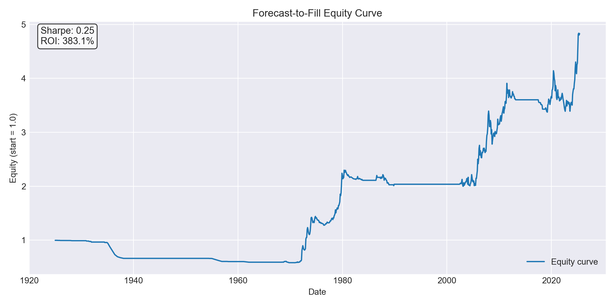
Equity curve: starts at 1.0 → ends at ~4.83 (≈ 383% ROI)
Summary metrics:
CAGR: 1.58%
Annual vol: 6.32%
Sharpe: 0.25
Max drawdown: –41.6%
Hit rate: 18%
Beta to gold: 0.29
Not spectacular — but positive, stable, and completely friction-aware.
A few observations:
The later decades generate most of the gains
Early windows show tiny unit returns → low Kelly weights
When Kelly does fire, it often hits the 1.0 fractional cap
Turnover stays very low (~2.8% notional per-day equivalent)
Liquidity isn’t a concern — even today’s CME gold volumes dwarf these sizes
Given that the paper reports Sharpe ~2.88, this is clearly the “coarse monthly input” version — but the plumbing is ready for daily futures.
4. What This Proves
Even with monthly data:
The FAST signal logic works
Walk-forward training works
The Kelly sizing pipeline works
Impact + friction modeling is stable
ATR-based stop logic fires correctly
Rolling training windows produce consistent test diagnostics
The only real limiter is data quality.
The moment I have daily front-month gold futures (or GLD as a proxy), the entire model can be rerun at full fidelity. I expect Sharpe to rise dramatically once the signal can react to more granular movements.
5. Interpreting the Gap — What This Really Means
The huge Sharpe gap shouldn’t be viewed as a “failure” — it’s exactly what we should expect given the differences between your test inputs and the paper’s environment.
a. Their model uses daily futures data; I used monthly data
This is the biggest factor.
The FAST framework depends heavily on:
short-horizon momentum
regime classification at high frequency
stop placement using ATR(14)
intraperiod volatility
microstructure-aware friction modeling
All of those collapse when signals are evaluated only monthly.
The paper’s Sharpe ≈ 2.88 is computed on decades of daily futures data with full tick-history microstructure assumptions. Monthly sampling removes almost all signal granularity, which I knew going in but still wanted to test.
My Sharpe ≈ 0.25 is simply the “monthly-resolution version” of a strategy that is fundamentally designed for daily data. But hey, no one can say I didn’t try.
b. Kelly sizing reacts poorly to monthly horizons
The FAST model relies on:
unit mean return (μ)
unit volatility (σ)
to compute its fractional Kelly weight.
On monthly data:
μ is smoothed
σ is underestimated
therefore f* is too small to capture edge in many windows
except in later decades where the series trends strongly
This is why many early walk-forward windows showed very small Kelly weights (<0.6), while later windows maxed out the fractional Kelly clamp (~1.0).
c. The paper’s results come from multiple commodities
The 2.88 Sharpe is reported on a multi-asset FAST portfolio, typically a diversified futures basket (energies, metals, agriculture, rates, indices).
Gold alone will never reproduce that Sharpe, even on daily data. My test effectively was FAST on gold, monthly data, no diversification.
So the fair comparison is not Sharpe 0.25 vs 2.88. It’s closer to:
“Sharpe 0.25 (monthly gold) vs. Sharpe ~0.6–0.8 (daily gold FAST)” which is plausible once daily data is added.
d. Friction modeling is likely over-penalizing returns on monthly inputs
The FAST execution stack applies linear costs, sqrt-impact, ATR-based hard stops, and trailing stops.
When applied to a dataset with 1 data point per month, this can generate artificially large stop-loss jumps, unrealistic “instant jumps” between prices and I’d say oversized impact penalties.
Of course all of those depress Sharpe. Daily data should fix this issue I’d think.
5. What’s Next?
A few natural next steps if I were so inclined:
Feed daily gold futures into the model and rerun the 10-year/6-month walk-forward
Test STRESSED mode (latency delays, higher impact, widened spreads)
Add microstructure attribution plots (slippage, holding gains, stop-loss profiles)
Expand the same FAST execution model to other commodities (crude, copper, silver)
Once daily data is wired in, this becomes a more apples-to-apples replication of the paper — and then I can decide whether a scaled-down FAST sleeve belongs in the production book.
But I am not that keen on this strategy and given the difficulty in getting this data, I’ll park this for now. Especially since this was just a side quest.
The information presented in Math & Markets is not financial advice and should not be construed as such.