
Synthetic Markets from Scratch: A Practical Guide to Stochastic Data Generation
Part 87 — How to build, calibrate, validate, and stress-test with market data that never existed

This post is based on an ask by one of my readers. This is also something I have previously experimented with: Retraining the Hybrid Ensemble on Synthetic Regimes // Stress-Testing V6 with Synthetic Markets (Part 1: Building the Stochastic Model) // Stress-Testing V6 with Synthetic Markets (Part 2: Results and Failure Modes)
I have previously written about building a synthetic SPY generator to stress-test a trading strategy against market scenarios that historical data simply doesn’t cover. The questions and responses I got were mostly variations of: “how did you actually build that thing?”
This post answers that question, properly, without the strategy context getting in the way. It is a standalone guide to synthetic financial data: the math behind the models, the code to implement them, the statistical tests to validate them, and the honest accounting of what synthetic data can and cannot do.
If you have ever asked “what if we got a crash that’s different from 2020?” or “how would this hold up in a 2000-style slow grind?”—this is the machinery that lets you answer those questions empirically rather than with hand-waving.
BLUF: If you are impatient and just want to get to the code, here you go:
1. Why Bother With Synthetic Data?
Before building anything, it is worth being precise about the problem synthetic data solves.
The standard backtesting approach runs a strategy against historical price series and reports performance metrics. This works reasonably well if the historical window contains enough variety, but in practice, it rarely does. A 2015–2025 window gives you exactly one flash crash, one sustained bear market, one rate-hiking cycle, and zero prolonged stagflation periods. If your strategy has never seen something, you have no evidence it handles it well or badly—you just have silence.
The academic literature sometimes calls this the Backtest Overfitting Problem. The more you tune a strategy to a specific historical dataset, the better it looks in-sample and the less informative that performance becomes about the future. Synthetic data provides a partial remedy: if the generator captures the statistical structure of real markets rather than their specific history, you can run your strategy against thousands of plausible futures and identify failure modes that no finite historical window can reveal.
There is an important caveat I will state now and return to at the end: synthetic data is excellent for stress-testing and scenario analysis, and much more dangerous as training data. Real price series carry information about actual economic relationships—information that stochastic simulators systematically omit. Use synthetic data for testing. Be very careful about training on it.
2. The Statistical Fingerprint of Real Markets
The generator needs to reproduce what real markets actually look like statistically. Before writing a single line of simulation code, it is worth cataloguing exactly which properties matter.
Using 30+ years of SPY daily returns, the key statistics shake out like this:
Property                    SPY (1993-2025)    Gaussian Assumption    Gap
──────────────────────────────────────────────────────────────────────────
Annualized Return             ~10.1%             N/A                  —
Annualized Volatility         ~18.7%             N/A                  —
Sharpe Ratio                  ~0.54              N/A                  —
Skewness                      -0.55              0.00                 Large
Excess Kurtosis               11.72              0.00                 Enormous
Lag-1 Autocorrelation         -0.08              0.00                 Moderate
Lag-1 Vol Autocorrelation      0.25              0.00                 Large
Tail Events (>3σ)              ~1.2%             0.27%                4× more
Each row in that table is a failure mode for naive Gaussian simulation. Let me explain why each one matters.
Skewness (-0.55): Returns are not symmetric. Large down days are more common than large up days of equivalent magnitude. A coin-flip model misses this entirely.
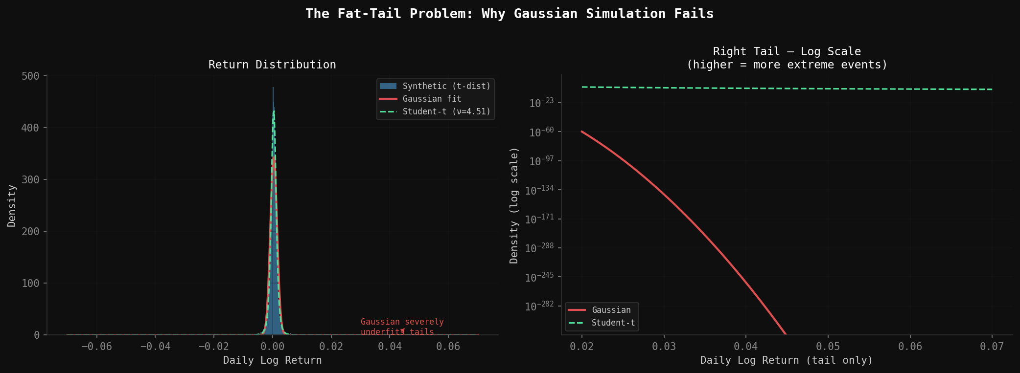
Excess kurtosis (11.72): This is the fat-tail signature. Under normality, a 3-sigma daily move should happen 0.27% of the time—about once every 380 trading days. In actual SPY data it happens closer to 1.2% of the time, or once every 83 days. Market crashes are not 10-sigma events that happen once a century; they are fat-tail events that happen every few years.
Lag-1 autocorrelation (-0.08): A weak but real negative serial correlation. Large up days slightly predict modest reversal, and vice versa. Markets exhibit short-term mean reversion alongside longer-term momentum.
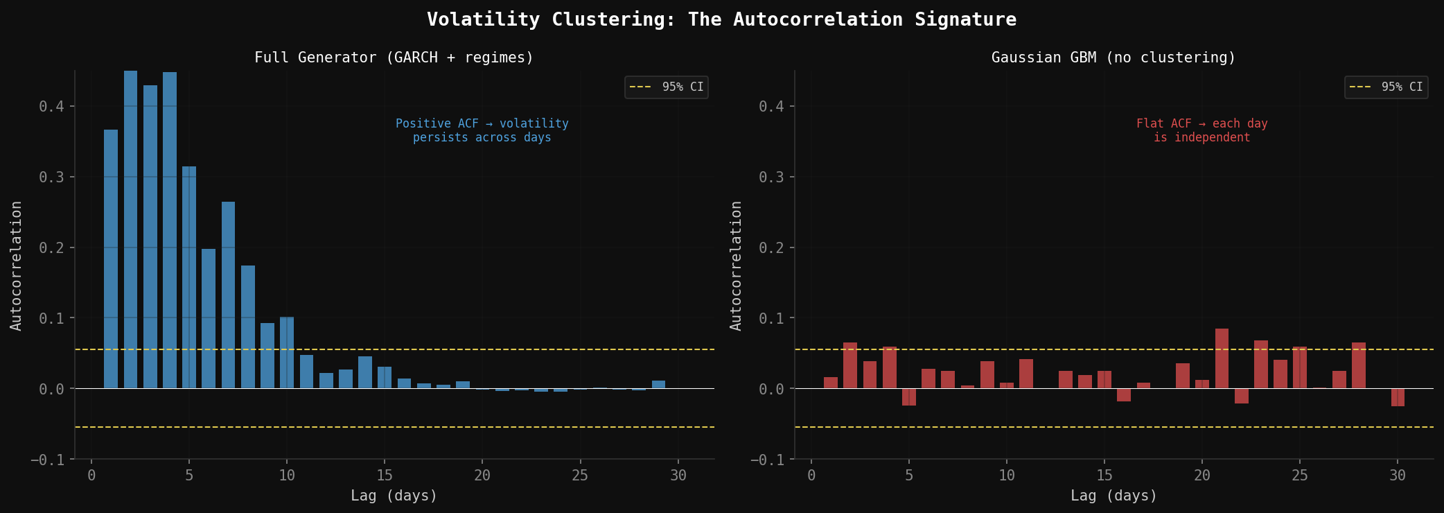
Lag-1 volatility autocorrelation (0.25): This is volatility clustering, and it is one of the most robust empirical facts in all of finance. Volatile periods tend to stay volatile. Calm periods tend to stay calm. A market that was turbulent yesterday is more likely to be turbulent tomorrow—not because of any predictive model, but just because that is how markets structurally behave.
Any synthetic generator that ignores these properties will produce price paths that look plausible in charts but fail immediately when you run statistical tests on them.
3. The Stochastic Model Stack
No single model captures all of these properties. The right approach is to build several models, each targeting specific statistical features, then combine them into a single generator.
3.1 The Baseline: Geometric Brownian Motion
GBM is where every quantitative finance course starts. The stochastic differential equation is:
dS = μS dt + σS dWHere S is price, μ is drift, σ is volatility, and dW is a Wiener process (standard Brownian motion increment). In discrete time over daily steps:
r_t = μ·Δt + σ·√Δt·Z_t

where Z_t ~ N(0,1)
GBM gets two things right: positive drift over time, and the intuition that percentage returns rather than absolute price changes should be normally distributed. It gets everything else wrong. Constant volatility, Gaussian tails, no serial correlation. But it is the skeleton on which everything else hangs.
import numpy as np
import pandas as pd
import matplotlib.pyplot as plt
from scipy import stats

def simulate_gbm(mu: float, sigma: float, S0: float, T: int, seed: int = 42) -> np.ndarray:
    """
    Simulate a single price path using Geometric Brownian Motion.

    mu:    Annual drift (e.g. 0.10 for 10%)
    sigma: Annual volatility (e.g. 0.187 for 18.7%)
    S0:    Starting price
    T:     Number of trading days

    Returns array of length T+1 (including starting price).
    """
    rng = np.random.default_rng(seed)
    dt = 1 / 252  # daily step

    daily_mu = mu * dt
    daily_sigma = sigma * np.sqrt(dt)

    log_returns = daily_mu - 0.5 * sigma**2 * dt + daily_sigma * rng.standard_normal(T)
    prices = S0 * np.exp(np.cumsum(np.insert(log_returns, 0, 0)))

    return prices
3.2 GARCH(1,1) for Volatility Clustering
GARCH (Generalized Autoregressive Conditional Heteroskedasticity) is the standard model for volatility clustering. The key insight is that tomorrow’s variance is a weighted combination of three things: a long-run baseline, today’s squared shock, and today’s estimated variance.
σ²_t = ω + α·ε²_(t-1) + β·σ²_(t-1)The parameters:
ω is the long-run variance floor (makes sure σ² never collapses to zero)
α (ARCH term) captures how strongly recent shocks feed into tomorrow’s variance
β (GARCH term) captures how strongly today’s estimated variance persists into tomorrow
For SPY, reasonable calibrated values are α = 0.09, β = 0.89. Their sum, α + β = 0.98, is close to 1—this is characteristic of high persistence, meaning volatility shocks decay slowly. After a 30% crash, it typically takes weeks for realized volatility to return to its baseline level. The GARCH model replicates this.
def simulate_garch(mu: float, omega: float, alpha: float, beta: float,
                   S0: float, T: int, seed: int = 42) -> tuple[np.ndarray, np.ndarray]:
    """
    Simulate price path with GARCH(1,1) volatility dynamics.

    Returns (prices, conditional_volatilities).
    """
    rng = np.random.default_rng(seed)
    dt = 1 / 252

    # Long-run variance implied by parameters
    long_run_var = omega / (1 - alpha - beta)

    variances = np.zeros(T)
    returns = np.zeros(T)
    variances[0] = long_run_var

    for t in range(T):
        # Draw return shock
        z = rng.standard_normal()
        returns[t] = mu * dt + np.sqrt(variances[t] * dt) * z

        # Update variance for next period
        epsilon_sq = (returns[t] - mu * dt) ** 2
        if t + 1 < T:
            variances[t+1] = omega + alpha * epsilon_sq / dt + beta * variances[t]

    prices = S0 * np.exp(np.cumsum(np.insert(returns, 0, 0)))
    vols = np.sqrt(variances * 252)  # annualize

    return prices[1:], vols


# SPY-calibrated parameters
omega_spy = 0.000002   # long-run daily variance floor
alpha_spy = 0.09
beta_spy  = 0.89
3.3 Fat Tails with the Student’s t Distribution
The simplest and most effective fix for fat tails is replacing the Gaussian noise term with draws from a Student’s t distribution. As degrees of freedom ν decreases, the tails get fatter. At ν → ∞, you recover the Gaussian.
The mapping between excess kurtosis and degrees of freedom is:
Excess Kurtosis = 6 / (ν - 4),    for ν > 4

Solving for ν:
ν = 6 / Excess_Kurtosis + 4
For SPY’s excess kurtosis of 11.72:
ν = 6 / 11.72 + 4 ≈ 4.51At ν = 4.51, extreme events occur roughly 4× more often than a Gaussian would predict—matching the empirical tail frequency in the historical data. The t-distribution also produces negative skew when combined with GBM drift dynamics, which partially addresses that -0.55 skewness signature.
def draw_fat_tail_shocks(T: int, nu: float, seed: int = 42) -> np.ndarray:
    """
    Draw T noise samples from a Student's t distribution scaled to unit variance.

    nu: degrees of freedom (lower = fatter tails)
        nu=4.51 matches SPY's excess kurtosis of ~11.7
        nu=6.0  matches moderate fat tails
        nu=30   is close to Gaussian
    """
    rng = np.random.default_rng(seed)

    # Student's t with variance = nu/(nu-2), normalize to unit variance
    raw = rng.standard_t(nu, size=T)
    scale = np.sqrt((nu - 2) / nu)

    return raw * scale


# Quick sanity check on tail properties
def report_tail_stats(shocks: np.ndarray, nu: float) -> None:
    kurtosis = stats.kurtosis(shocks)
    theoretical_excess_kurtosis = 6 / (nu - 4) if nu > 4 else float('inf')
    tail_prob = np.mean(np.abs(shocks) > 3)

    print(f"Degrees of freedom:          {nu:.2f}")
    print(f"Empirical excess kurtosis:   {kurtosis:.2f}")
    print(f"Theoretical excess kurtosis: {theoretical_excess_kurtosis:.2f}")
    print(f"Empirical |Z| > 3 prob:      {tail_prob:.4f}  (Gaussian: 0.0027)")
3.4 Mean Reversion with the Ornstein-Uhlenbeck Process
The Ornstein-Uhlenbeck (OU) process is the standard continuous-time mean-reverting model:
dX = θ(μ - X) dt + σ dWHere θ controls the speed of mean reversion—how strongly deviations from μ get pulled back. In discrete time:
X_t = X_(t-1) + θ(μ - X_(t-1))·Δt + σ·√Δt·Z_tFor equity returns, the mean-reversion component is subtle (the lag-1 autocorrelation of -0.08 implies θ is small). For VIX, mean reversion is much more pronounced—VIX always drifts back toward its long-run average of ~18, even after spikes to 80.
def simulate_ou_process(theta: float, mu: float, sigma: float,
                         X0: float, T: int, seed: int = 42) -> np.ndarray:
    """
    Simulate Ornstein-Uhlenbeck mean-reverting process.

    theta: mean-reversion speed (higher = faster reversion)
    mu:    long-run mean
    sigma: diffusion coefficient
    X0:    starting value
    T:     number of steps

    Useful for VIX simulation, interest rates, or adding mean-reversion
    adjustment to equity return models.
    """
    rng = np.random.default_rng(seed)
    dt = 1 / 252

    path = np.zeros(T + 1)
    path[0] = X0

    for t in range(T):
        drift = theta * (mu - path[t]) * dt
        diffusion = sigma * np.sqrt(dt) * rng.standard_normal()
        path[t + 1] = path[t] + drift + diffusion

    return path


# VIX-calibrated OU parameters
vix_theta = 4.5    # moderately fast mean reversion
vix_mu    = 18.0   # long-run VIX average
vix_sigma = 25.0   # high diffusion (VIX is volatile itself)
3.5 Regime Switching with a Markov Chain
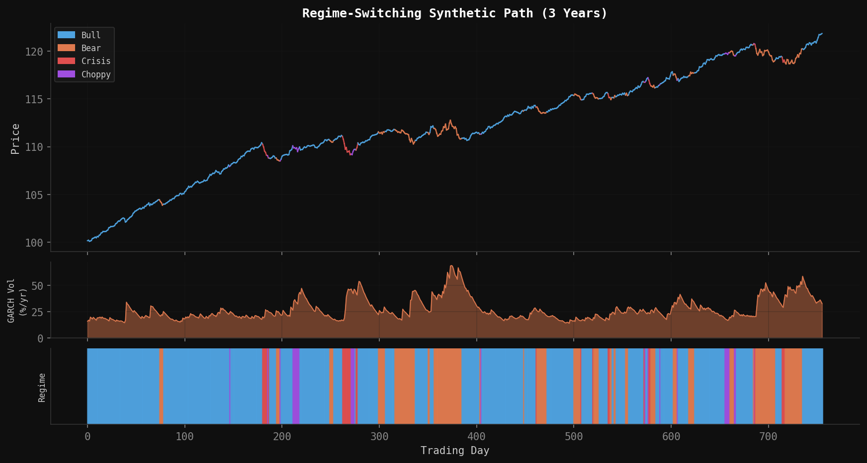
The most powerful addition to the model is regime switching. Real markets cycle through meaningfully different states—calm bull markets, panicked crashes, grinding bear markets, choppy sideways periods—and each regime has its own return and volatility characteristics.
The Markov chain assumption is that tomorrow’s regime depends only on today’s regime (not on the full history), with fixed transition probabilities. Estimated from SPY data, the regime distribution and transition matrix look like this:
Regime Distribution:
────────────────────────────────────────────────────────────
Regime       Base Freq    Annual Drift    Daily Volatility
────────────────────────────────────────────────────────────
Bull          48.3%         +15%              0.7%
Bear          19.5%         -12%              1.3%
Crisis         6.2%         -35%              2.5%
Choppy        26.0%          +2%              1.5%

Transition Matrix (rows = current, cols = next):
──────────────────────────────────────────────────────
From/To       Bull    Bear    Crisis    Choppy
──────────────────────────────────────────────
Bull          0.95    0.03    0.01      0.01
Bear          0.10    0.85    0.03      0.02
Crisis        0.15    0.25    0.55      0.05
Choppy        0.20    0.15    0.05      0.60
The diagonal dominance reflects persistence—once in a regime, you tend to stay there. But crisis regimes are inherently unstable (diagonal of only 0.55), reflecting the empirical observation that crashes don’t last forever.
import numpy as np

# Regime parameters
REGIME_PARAMS = {
    # regime_id: (annual_drift, daily_vol, name)
    0: (0.15,  0.007, 'Bull'),
    1: (-0.12, 0.013, 'Bear'),
    2: (-0.35, 0.025, 'Crisis'),
    3: (0.02,  0.015, 'Choppy'),
}

# Calibrated transition matrix
TRANSITION_MATRIX = np.array([
    [0.95, 0.03, 0.01, 0.01],  # from Bull
    [0.10, 0.85, 0.03, 0.02],  # from Bear
    [0.15, 0.25, 0.55, 0.05],  # from Crisis
    [0.20, 0.15, 0.05, 0.60],  # from Choppy
])

def simulate_regime_sequence(T: int, initial_regime: int = 0,
                              seed: int = 42) -> np.ndarray:
    """
    Simulate a sequence of regime labels using a Markov chain.
    Returns array of regime indices, length T.
    """
    rng = np.random.default_rng(seed)
    regimes = np.zeros(T, dtype=int)
    regimes[0] = initial_regime

    for t in range(1, T):
        current = regimes[t - 1]
        regimes[t] = rng.choice(4, p=TRANSITION_MATRIX[current])

    return regimes
4. Assembling the Full Generator
Now we combine all five components into a single function. The execution order matters:
Draw the regime sequence from the Markov chain
For each day, look up that regime’s drift and base volatility
Apply the GARCH update to get the conditional volatility
Draw the return shock from Student’s t (not Gaussian)
Add a small mean-reversion adjustment
Compute the price change via GBM dynamics
import numpy as np
import pandas as pd
from scipy import stats


class SyntheticMarketGenerator:
    """
    Full stochastic market generator combining:
    - Regime-switching Markov chain
    - GARCH(1,1) volatility dynamics
    - Student's t fat tails
    - Ornstein-Uhlenbeck mean reversion
    - GBM baseline
    """

    def __init__(
        self,
        # GBM baseline
        mu: float = 0.10,
        sigma: float = 0.187,
        # GARCH
        garch_omega: float = 2e-6,
        garch_alpha: float = 0.09,
        garch_beta: float = 0.89,
        # Fat tails
        t_nu: float = 4.51,
        # Mean reversion
        mr_theta: float = 0.08,
        # Regime switching
        use_regimes: bool = True,
        transition_matrix: np.ndarray = None,
        regime_params: dict = None,
    ):
        self.mu = mu
        self.sigma = sigma
        self.garch_omega = garch_omega
        self.garch_alpha = garch_alpha
        self.garch_beta = garch_beta
        self.t_nu = t_nu
        self.mr_theta = mr_theta
        self.use_regimes = use_regimes

        self.transition_matrix = transition_matrix if transition_matrix is not None else \
            np.array([
                [0.95, 0.03, 0.01, 0.01],
                [0.10, 0.85, 0.03, 0.02],
                [0.15, 0.25, 0.55, 0.05],
                [0.20, 0.15, 0.05, 0.60],
            ])

        self.regime_params = regime_params if regime_params is not None else {
            0: {'drift': 0.15,  'vol_mult': 0.7,  'name': 'Bull'},
            1: {'drift': -0.12, 'vol_mult': 1.3,  'name': 'Bear'},
            2: {'drift': -0.35, 'vol_mult': 2.5,  'name': 'Crisis'},
            3: {'drift': 0.02,  'vol_mult': 1.5,  'name': 'Choppy'},
        }

    def generate(
        self,
        T: int = 252,
        S0: float = 100.0,
        initial_regime: int = 0,
        seed: int = 42,
    ) -> pd.DataFrame:
        """
        Generate T days of synthetic price data.

        Returns DataFrame with columns:
            price, daily_return, log_return, regime, regime_name,
            conditional_vol (annualized), garch_var
        """
        rng = np.random.default_rng(seed)
        dt = 1 / 252

        # --- Step 1: regime sequence ---
        regimes = np.zeros(T, dtype=int)
        regimes[0] = initial_regime
        if self.use_regimes:
            for t in range(1, T):
                regimes[t] = rng.choice(4, p=self.transition_matrix[regimes[t - 1]])

        # --- Step 2: GARCH variance initialization ---
        long_run_var = self.garch_omega / (1 - self.garch_alpha - self.garch_beta)
        garch_var = np.zeros(T)
        garch_var[0] = long_run_var

        # --- Step 3: Draw fat-tail shocks ---
        raw_shocks = rng.standard_t(self.t_nu, size=T)
        shocks = raw_shocks * np.sqrt((self.t_nu - 2) / self.t_nu)  # unit variance

        # --- Step 4: Build returns ---
        log_returns = np.zeros(T)
        prev_log_return = 0.0

        for t in range(T):
            regime = regimes[t]
            regime_drift = self.regime_params[regime]['drift'] if self.use_regimes else self.mu
            regime_vol_mult = self.regime_params[regime]['vol_mult'] if self.use_regimes else 1.0

            # Effective daily volatility from GARCH, scaled by regime
            daily_vol = np.sqrt(garch_var[t] * dt) * regime_vol_mult
            daily_vol = max(daily_vol, 0.001)  # floor at 0.1% to prevent collapse

            # Mean reversion component (pulls return toward zero after extremes)
            mr_adj = -self.mr_theta * prev_log_return * dt

            # GBM drift term for this regime
            drift_term = regime_drift * dt - 0.5 * (daily_vol ** 2)

            # Combined return
            log_returns[t] = drift_term + daily_vol * shocks[t] + mr_adj
            prev_log_return = log_returns[t]

            # GARCH update for next period
            if t + 1 < T:
                epsilon_sq = (log_returns[t] - regime_drift * dt) ** 2
                garch_var[t + 1] = (
                    self.garch_omega
                    + self.garch_alpha * epsilon_sq / dt
                    + self.garch_beta * garch_var[t]
                )
                garch_var[t + 1] = max(garch_var[t + 1], 1e-8)

        # --- Step 5: Construct price series ---
        prices = S0 * np.exp(np.cumsum(log_returns))
        daily_returns = np.exp(log_returns) - 1

        df = pd.DataFrame({
            'price':           prices,
            'daily_return':    daily_returns,
            'log_return':      log_returns,
            'regime':          regimes,
            'regime_name':     [self.regime_params[r]['name'] for r in regimes],
            'conditional_vol': np.sqrt(garch_var * 252),
            'garch_var':       garch_var,
        })
        df.index.name = 'day'

        return df


# Basic usage
gen = SyntheticMarketGenerator()
df = gen.generate(T=252, S0=450.0, seed=99)
print(df.head(10))
print(f"\nTotal return: {(df['price'].iloc[-1] / df['price'].iloc[0] - 1) * 100:.1f}%")
print(f"Max drawdown: {((df['price'] / df['price'].cummax()) - 1).min() * 100:.1f}%")
5. Generating Correlated Multi-Asset Paths
A single synthetic SPY path is not very useful on its own. Real trading strategies involve multiple assets with specific correlation structures. The standard approach is Cholesky decomposition of the correlation matrix.
If you have assets with correlations described by matrix Σ, and you want correlated shocks Z₁, Z₂, ..., Zₙ, you compute the Cholesky factor L such that LLᵀ = Σ, then generate independent standard normals W and multiply: Z = LW.
For a three-asset portfolio (equity index, long-term bonds, VIX), calibrated correlations look like:
            Equity    Bonds    VIX
Equity       1.00     -0.40   -0.75
Bonds       -0.40      1.00    0.30
VIX         -0.75      0.30    1.00
The equity-VIX correlation of -0.75 is the most important: when stocks fall, fear spikes. The equity-bond correlation of -0.40 captures the flight-to-quality dynamic. These correlations are not fixed in practice—they tend to strengthen during crises—but as a baseline they are reasonable.
def generate_correlated_paths(
    T: int = 252,
    corr_matrix: np.ndarray = None,
    asset_params: list[dict] = None,
    seed: int = 42,
) -> pd.DataFrame:
    """
    Generate correlated synthetic paths for multiple assets.

    corr_matrix: (n x n) correlation matrix
    asset_params: list of dicts with keys 'name', 'mu', 'sigma', 'S0'

    Returns DataFrame with one column per asset (prices).
    """
    if corr_matrix is None:
        corr_matrix = np.array([
            [ 1.00, -0.40, -0.75],
            [-0.40,  1.00,  0.30],
            [-0.75,  0.30,  1.00],
        ])

    if asset_params is None:
        asset_params = [
            {'name': 'SPY',  'mu': 0.10,  'sigma': 0.187, 'S0': 450.0},
            {'name': 'TLT',  'mu': 0.04,  'sigma': 0.150, 'S0': 95.0},
            {'name': 'VIX',  'mu': 0.00,  'sigma': 0.800, 'S0': 18.0},
        ]

    rng = np.random.default_rng(seed)
    n_assets = len(asset_params)
    dt = 1 / 252

    # Cholesky decomposition for correlated shocks
    L = np.linalg.cholesky(corr_matrix)

    # Independent normals -> correlated
    independent = rng.standard_normal((T, n_assets))
    correlated = (L @ independent.T).T  # shape (T, n_assets)

    prices = np.zeros((T + 1, n_assets))
    for i, params in enumerate(asset_params):
        prices[0, i] = params['S0']

    for t in range(T):
        for i, params in enumerate(asset_params):
            mu, sigma = params['mu'], params['sigma']
            log_ret = (mu - 0.5 * sigma**2) * dt + sigma * np.sqrt(dt) * correlated[t, i]
            prices[t + 1, i] = prices[t, i] * np.exp(log_ret)

    df = pd.DataFrame(
        prices[1:],
        columns=[p['name'] for p in asset_params],
    )
    df.index.name = 'day'

    return df


# Generate and inspect correlations
paths = generate_correlated_paths(T=252, seed=42)
log_rets = np.log(paths / paths.shift(1)).dropna()
print("Realized correlations:")
print(log_rets.corr().round(2))
6. Adding Synthetic VIX
VIX deserves special treatment because it is not a price series—it is a volatility index with specific structural properties. It is mean-reverting (always drifts back toward ~18), spikes sharply during equity drawdowns (negative correlation with returns), and has a strong asymmetry: it rises faster than it falls.
The jump-diffusion extension of the OU process captures this:
dVIX = κ(V̄ - VIX)dt + σ_VIX·dW + J·dNwhere dN is a Poisson jump process that fires when equity returns exceed a negative threshold, and J is the jump size (calibrated to the typical VIX spike magnitude of 8–15 points).
def simulate_vix(
    equity_returns: np.ndarray,
    kappa: float = 4.5,       # mean reversion speed
    vbar: float = 18.0,       # long-run mean
    sigma_vix: float = 4.0,   # diffusion coefficient
    vix0: float = 18.0,       # starting VIX
    jump_threshold: float = -0.02,    # equity return that triggers jump
    jump_mean: float = 10.0,          # average VIX jump size
    jump_std: float = 3.0,            # jump size dispersion
    seed: int = 42,
) -> np.ndarray:
    """
    Simulate VIX path given realized equity returns.

    VIX spikes when equity returns fall below jump_threshold,
    and mean-reverts toward vbar otherwise.
    """
    rng = np.random.default_rng(seed)
    T = len(equity_returns)
    dt = 1 / 252

    vix = np.zeros(T + 1)
    vix[0] = vix0

    for t in range(T):
        # Mean reversion drift
        drift = kappa * (vbar - vix[t]) * dt

        # Diffusion
        diffusion = sigma_vix * np.sqrt(dt) * rng.standard_normal()

        # Jump if equity crash
        jump = 0.0
        if equity_returns[t] < jump_threshold:
            severity = abs(equity_returns[t]) / abs(jump_threshold)
            jump_size = rng.normal(jump_mean * severity, jump_std)
            jump = max(jump_size, 0)  # VIX can only jump up, not down

        vix[t + 1] = max(vix[t] + drift + diffusion + jump, 5.0)  # floor at 5

    return vix[1:]


# Pair with equity returns
gen = SyntheticMarketGenerator()
equity_df = gen.generate(T=252, seed=42)
vix_series = simulate_vix(equity_df['daily_return'].values, seed=42)

equity_df['vix'] = vix_series

print(f"VIX range: {vix_series.min():.1f} - {vix_series.max():.1f}")
print(f"VIX mean:  {vix_series.mean():.1f}")
print(f"Corr(equity returns, VIX changes): "
      f"{np.corrcoef(equity_df['daily_return'], np.diff(vix_series, prepend=vix_series[0]))[0,1]:.2f}")
7. Scenario Engineering
The power of synthetic data is not just generating “random” markets—it is generating specific market conditions to probe strategy behavior. Scenario engineering means overriding the base generator’s parameters to produce targeted environments.
Here are eight canonical scenarios with the specific parameter modifications that create them:
SCENARIOS = {
    'crash': {
        'description': 'Sudden equity crash with gradual recovery',
        'override': {
            'initial_regime': 2,  # start in Crisis
            'transition_override': {
                # Keep crisis regime sticky for first 40 days,
                # then force transition toward Bear/Bull recovery
            },
        },
        'drift_override': None,  # use regime drift
        'vol_override': None,
    },

    'choppy': {
        'description': 'High volatility, no directional trend',
        'mu_override': 0.02,
        'sigma_override': 0.35,
    },

    'stagflation': {
        'description': 'Slow grind down with moderate vol',
        'mu_override': -0.08,
        'sigma_override': 0.15,
    },

    'bull': {
        'description': 'Strong sustained uptrend',
        'mu_override': 0.20,
        'sigma_override': 0.12,
    },

    'slow_bleed': {
        'description': 'Gradual decline, low volatility (momentum killers)',
        'mu_override': -0.105,
        'sigma_override': 0.12,
    },

    'flash_crash': {
        'description': 'Sharp V-shaped crash and rapid recovery',
        'crash_days': 10,
        'crash_magnitude': -0.37,
        'recovery_days': 20,
    },

    'sideways': {
        'description': 'Range-bound market, high mean reversion',
        'mu_override': 0.00,
        'sigma_override': 0.10,
        'mr_theta_override': 0.50,
    },

    'bear': {
        'description': 'Sustained bear market with elevated vol',
        'mu_override': -0.15,
        'sigma_override': 0.25,
    },
}


def generate_scenario(
    scenario_name: str,
    T: int = 252,
    S0: float = 100.0,
    seed: int = 42,
) -> pd.DataFrame:
    """
    Generate a scenario-specific price path.
    """
    if scenario_name not in SCENARIOS:
        raise ValueError(f"Unknown scenario: {scenario_name}. "
                         f"Choose from {list(SCENARIOS.keys())}")

    scenario = SCENARIOS[scenario_name]

    if scenario_name == 'flash_crash':
        return _generate_flash_crash(
            T=T, S0=S0,
            crash_days=scenario['crash_days'],
            crash_magnitude=scenario['crash_magnitude'],
            recovery_days=scenario['recovery_days'],
            seed=seed,
        )

    # For standard scenarios, override generator parameters
    gen = SyntheticMarketGenerator(
        mu=scenario.get('mu_override', 0.10),
        sigma=scenario.get('sigma_override', 0.187),
        mr_theta=scenario.get('mr_theta_override', 0.08),
        use_regimes=False,  # fixed parameters override regime switching
    )
    return gen.generate(T=T, S0=S0, seed=seed)


def _generate_flash_crash(
    T: int, S0: float,
    crash_days: int, crash_magnitude: float,
    recovery_days: int, seed: int,
) -> pd.DataFrame:
    """
    Inject a programmatic flash crash into an otherwise normal path.
    """
    gen = SyntheticMarketGenerator(mu=0.10, sigma=0.12, use_regimes=False)
    df = gen.generate(T=T, S0=S0, seed=seed)

    crash_start = T // 4
    crash_end = crash_start + crash_days
    recovery_end = crash_end + recovery_days

    pre_crash_price = df['price'].iloc[crash_start - 1]
    post_crash_price = pre_crash_price * (1 + crash_magnitude)

    # Inject crash: linear decline over crash_days
    crash_prices = np.linspace(pre_crash_price, post_crash_price, crash_days)
    df.loc[crash_start:crash_end - 1, 'price'] = crash_prices

    # Inject recovery: exponential recovery over recovery_days
    if recovery_end <= T:
        recovery_prices = np.linspace(post_crash_price, pre_crash_price, recovery_days)
        df.loc[crash_end:recovery_end - 1, 'price'] = recovery_prices

    return df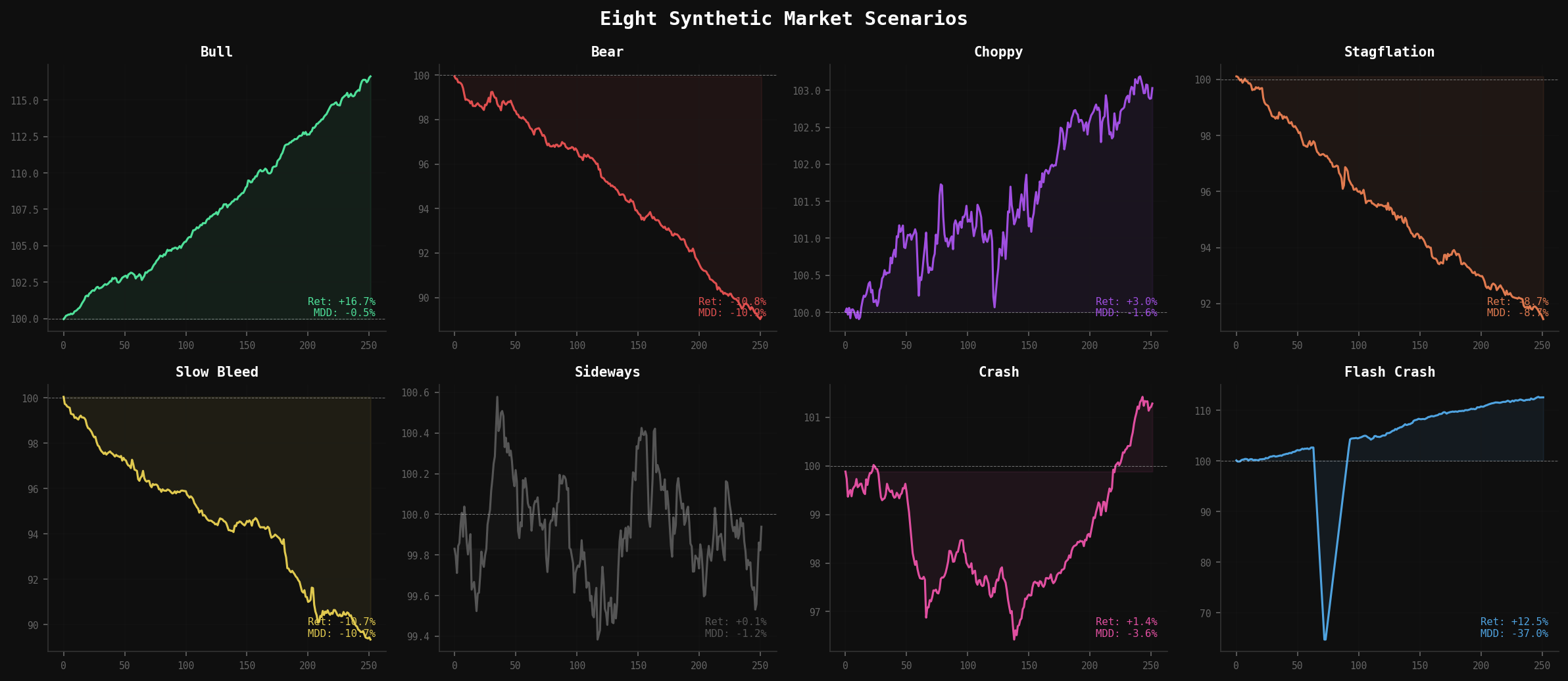
8. Generating From the Original Time Series: Bootstrap Methods
Everything in the previous sections builds a parametric generator: fit a model to historical data, then simulate from that model. The advantage is you can extrapolate beyond what history actually contains—generate crashes deeper than 2020, recoveries faster than 2020, volatility regimes that haven’t occurred yet.
The disadvantage is that the synthetic data is only as good as the model’s assumptions. If the GARCH parameters are slightly mis-calibrated, or the regime transition matrix is wrong, the synthetic returns won’t actually match the properties of the real series. You’re testing against your model’s world, not the real world’s world.
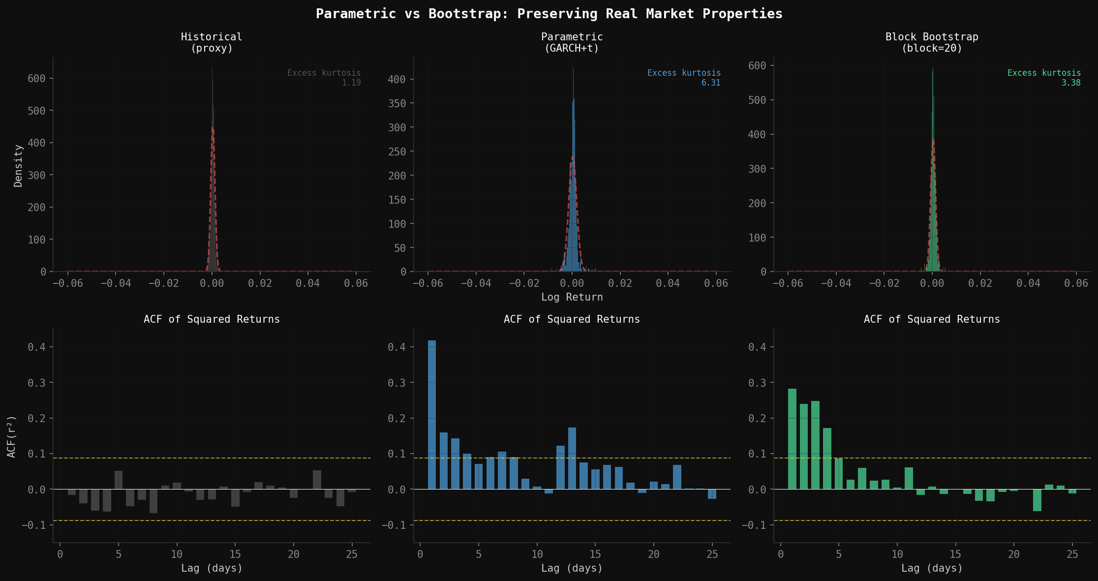
The alternative is resampling directly from the original time series. No distributional assumptions. No parameter estimation. The synthetic paths are built from actual historical returns, rearranged—so the fat tails, volatility clustering, and skewness are all preserved by construction, because you never left the empirical distribution.
8.1 Why Not Just Shuffle Returns?
The naive version — shuffle all daily returns randomly — breaks immediately (and trust me, I’ve tried this). It destroys the autocorrelation structure that makes markets behave like markets. Volatility clustering disappears because high-vol days are no longer adjacent to other high-vol days. Mean reversion disappears for the same reason. A shuffled return series has the right unconditional distribution but none of the right conditional dynamics.
The fix is block bootstrap: instead of resampling individual days, resample contiguous blocks of days. A block of 20 consecutive returns carries the local autocorrelation structure with it—if day 1 of the block was a high-vol day, day 2 is still the high-vol day that historically followed it. Piece enough blocks together and you get a path that has the right unconditional distribution and approximately preserves short-run dynamics.
8.2 Choosing Block Length
Block length is the key tuning parameter and it involves a direct tradeoff:
Too short (e.g. 1–3 days): autocorrelation structure breaks down, approaches naive shuffle
Too long (e.g. 100+ days): you’re just stitching together large chunks of actual history, which limits diversity across paths
Sweet spot: roughly the persistence horizon of the dependency you care about
For equity returns, volatility clustering persists for about 10–20 trading days (matching GARCH’s typical half-life). A block length of 15–20 days is a reasonable default. For strategies with longer lookback windows, you’d want longer blocks.
The stationary bootstrap (Politis & Romano, 1994) is a refinement: instead of fixed block length, each block’s length is drawn from a geometric distribution with mean equal to your target block length. This prevents artificial periodicity at block boundaries and makes the resampled series stationary by construction.
import numpy as np
import pandas as pd


def block_bootstrap(
    returns: np.ndarray,
    T: int = 252,
    block_length: int = 20,
    S0: float = 100.0,
    seed: int = 42,
) -> pd.DataFrame:
    """
    Generate a synthetic price path by circular block bootstrap.

    Resamples contiguous blocks of actual returns to preserve
    short-run autocorrelation structure (volatility clustering,
    mean reversion) without any parametric assumptions.

    Parameters
    ----------
    returns      : Array of historical daily log returns
    T            : Number of days to generate
    block_length : Length of each resampled block (default: 20)
    S0           : Starting price
    seed         : RNG seed

    Returns
    -------
    pd.DataFrame with columns: price, log_return
    """
    rng = np.random.default_rng(seed)
    n = len(returns)
    synthetic_returns = np.zeros(T)
    t = 0

    while t < T:
        # Draw a random start index (circular — wraps around end of series)
        start = rng.integers(0, n)
        block = np.array([returns[(start + i) % n] for i in range(block_length)])

        # Clip to remaining days needed
        remaining = T - t
        block = block[:remaining]
        synthetic_returns[t:t + len(block)] = block
        t += len(block)

    prices = S0 * np.exp(np.cumsum(synthetic_returns))

    return pd.DataFrame({
        'price':      prices,
        'log_return': synthetic_returns,
    })


def stationary_bootstrap(
    returns: np.ndarray,
    T: int = 252,
    mean_block_length: int = 20,
    S0: float = 100.0,
    seed: int = 42,
) -> pd.DataFrame:
    """
    Generate a synthetic price path via stationary bootstrap.

    Block lengths are drawn from Geometric(1/mean_block_length),
    making the resampled series stationary and avoiding artificial
    periodicity at fixed block boundaries.

    Parameters
    ----------
    returns           : Array of historical daily log returns
    T                 : Number of days to generate
    mean_block_length : Expected block length (Geometric distribution mean)
    S0                : Starting price
    seed              : RNG seed

    Returns
    -------
    pd.DataFrame with columns: price, log_return
    """
    rng = np.random.default_rng(seed)
    n = len(returns)
    p = 1.0 / mean_block_length  # Geometric distribution parameter

    synthetic_returns = np.zeros(T)
    t = 0

    while t < T:
        start = rng.integers(0, n)
        # Geometric block length
        block_len = rng.geometric(p)
        block = np.array([returns[(start + i) % n] for i in range(block_len)])

        remaining = T - t
        block = block[:remaining]
        synthetic_returns[t:t + len(block)] = block
        t += len(block)

    prices = S0 * np.exp(np.cumsum(synthetic_returns))

    return pd.DataFrame({
        'price':      prices,
        'log_return': synthetic_returns,
    })
8.3 Strategy-Specific Property Selection
Here is where most synthetic data guides go wrong: they validate the generator against a generic list of statistical moments and call it done. But the properties that matter are the ones your specific strategy depends on.
Different strategy types are sensitive to entirely different statistical features:
Strategy Type          Properties That Matter Most
──────────────────────────────────────────────────────────────────────
Momentum / trend       Autocorrelation at your lookback horizon
                       Regime persistence (how long trends last)
                       Tail asymmetry (crash magnitude vs recovery speed)

Mean reversion         Half-life of deviations from mean
                       Vol-of-vol (does vol itself revert quickly?)
                       Bid-ask spread / transaction cost sensitivity

Vol targeting          GARCH persistence (α + β)
                       Vol-of-vol (realized vol of realized vol)
                       Correlation stability across vol regimes

Regime switching       Regime transition probabilities
                       Regime duration distributions
                       In-regime return and vol parameters

Pairs / stat arb       Cointegration stability
                       Spread mean and variance stationarity
                       Correlation breakdown frequency in stress
Before accepting a synthetic series as a valid test environment for your strategy, verify it preserves the properties your strategy actually uses. For a momentum strategy, that means checking autocorrelation at your signal’s lookback horizon. For a vol-targeting strategy, that means checking GARCH persistence. Generic moment-matching (mean, vol, kurtosis) is necessary but not sufficient.
def validate_for_strategy(
    synthetic_returns: np.ndarray,
    real_returns: np.ndarray,
    strategy_type: str = 'momentum',
) -> dict:
    """
    Validate synthetic returns against the properties most relevant
    to a specific strategy type.

    Parameters
    ----------
    synthetic_returns : Synthetic daily log return array
    real_returns      : Historical daily log return array
    strategy_type     : One of 'momentum', 'mean_reversion', 'vol_targeting'

    Returns
    -------
    dict of property name -> (real_value, synthetic_value, gap)
    """
    from scipy import stats

    results = {}

    def _acf(r, lag):
        return pd.Series(r).autocorr(lag=lag)

    def _half_life(r):
        # Estimate OU half-life from lag-1 autocorrelation
        lag1 = _acf(r, 1)
        if lag1 >= 1 or lag1 <= 0:
            return float('inf')
        return -np.log(2) / np.log(lag1)

    def _garch_persistence(r):
        # Proxy: lag-1 autocorrelation of squared returns
        # True GARCH fit would give alpha + beta directly
        return _acf(r ** 2, 1)

    if strategy_type == 'momentum':
        for lag in [1, 5, 10, 20]:
            real_acf = _acf(real_returns, lag)
            synth_acf = _acf(synthetic_returns, lag)
            results[f'acf_lag{lag}'] = (real_acf, synth_acf, synth_acf - real_acf)

        # Tail asymmetry: ratio of worst 5% days to best 5% days
        real_asym = np.percentile(real_returns, 5) / np.percentile(real_returns, 95)
        synth_asym = np.percentile(synthetic_returns, 5) / np.percentile(synthetic_returns, 95)
        results['tail_asymmetry'] = (real_asym, synth_asym, synth_asym - real_asym)

    elif strategy_type == 'mean_reversion':
        real_hl = _half_life(real_returns)
        synth_hl = _half_life(synthetic_returns)
        results['half_life_days'] = (real_hl, synth_hl, synth_hl - real_hl)

        # Vol of vol
        real_vov = pd.Series(real_returns).rolling(20).std().std()
        synth_vov = pd.Series(synthetic_returns).rolling(20).std().std()
        results['vol_of_vol'] = (real_vov, synth_vov, synth_vov - real_vov)

    elif strategy_type == 'vol_targeting':
        real_persist = _garch_persistence(real_returns)
        synth_persist = _garch_persistence(synthetic_returns)
        results['garch_persistence_proxy'] = (real_persist, synth_persist,
                                               synth_persist - real_persist)

        real_vov = pd.Series(real_returns).rolling(20).std().std()
        synth_vov = pd.Series(synthetic_returns).rolling(20).std().std()
        results['vol_of_vol'] = (real_vov, synth_vov, synth_vov - real_vov)

    print(f"\nStrategy-specific validation ({strategy_type})")
    print(f"{'Property':<28} {'Real':>10} {'Synthetic':>10} {'Gap':>10}")
    print('─' * 62)
    for prop, (r, s, gap) in results.items():
        print(f"{prop:<28} {r:>10.4f} {s:>10.4f} {gap:>+10.4f}")

    return results
8.4 Stationarity Checks
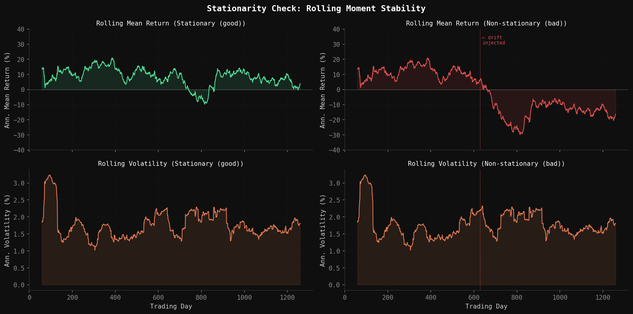
“Stable properties” means more than just matching moments globally. It means the statistical properties don’t drift across the simulation window. A synthetic series where volatility is high in the first half and low in the second half has the right unconditional variance but will produce misleading strategy test results—especially for strategies with rolling lookback windows that will see a structurally different environment as they move through the path.
The standard test is the Augmented Dickey-Fuller (ADF) test for unit roots. A stationary series—one whose statistical properties don’t change over time—should reject the null hypothesis of a unit root. For log returns (not prices), stationarity is almost always satisfied. But it is worth checking, especially on synthetic series generated with strong regime drift.
A second check is rolling moment stability: compute mean, variance, and skewness in rolling windows across the synthetic path and verify they don’t trend systematically.
from statsmodels.tsa.stattools import adfuller


def check_stationarity(
    returns: np.ndarray,
    label: str = 'Synthetic',
    window: int = 60,
) -> dict:
    """
    Check stationarity of a synthetic return series.

    Runs the Augmented Dickey-Fuller test and plots rolling
    mean and volatility to detect systematic drift.

    Parameters
    ----------
    returns : Daily return array
    label   : Display name
    window  : Rolling window for moment stability check (days)

    Returns
    -------
    dict with ADF results and rolling stability metrics.
    """
    import matplotlib.pyplot as plt

    # ADF test
    adf_result = adfuller(returns, autolag='AIC')
    adf_stat, p_value, _, _, critical_values, _ = adf_result

    print(f"\nStationarity check: {label}")
    print(f"  ADF statistic : {adf_stat:.4f}")
    print(f"  p-value       : {p_value:.4f}")
    print(f"  Critical (5%) : {critical_values['5%']:.4f}")
    if p_value < 0.05:
        print(f"  Result        : ✓ Stationary (reject unit root)")
    else:
        print(f"  Result        : ✗ Non-stationary — check for drift in synthetic series")

    # Rolling moment stability
    s = pd.Series(returns)
    rolling_mean = s.rolling(window).mean() * 252        # annualised
    rolling_vol = s.rolling(window).std() * np.sqrt(252) # annualised

    # Drift metric: max rolling mean minus min rolling mean (should be small)
    mean_drift = rolling_mean.dropna().max() - rolling_mean.dropna().min()
    vol_drift = rolling_vol.dropna().max() - rolling_vol.dropna().min()

    print(f"  Rolling mean drift (ann.) : {mean_drift * 100:.2f}%  "
          f"{'✓ stable' if mean_drift < 0.10 else '✗ drifting'}")
    print(f"  Rolling vol drift  (ann.) : {vol_drift * 100:.2f}%  "
          f"{'✓ stable' if vol_drift < 0.15 else '✗ drifting'}")

    # Plot rolling stability
    fig, axes = plt.subplots(2, 1, figsize=(12, 6), sharex=True)
    fig.suptitle(f'Rolling Moment Stability: {label}', fontsize=12)

    axes[0].plot(rolling_mean * 100, color='steelblue', lw=1)
    axes[0].axhline(0, color='black', lw=0.5, linestyle='--')
    axes[0].set_ylabel('Rolling Mean Return (%, ann.)')
    axes[0].set_title(f'{window}-day rolling annualised mean')

    axes[1].plot(rolling_vol * 100, color='darkorange', lw=1)
    axes[1].set_ylabel('Rolling Volatility (%, ann.)')
    axes[1].set_title(f'{window}-day rolling annualised volatility')
    axes[1].set_xlabel('Day')

    plt.tight_layout()
    plt.savefig(f'stationarity_{label.lower().replace(" ", "_")}.png',
                dpi=150, bbox_inches='tight')
    plt.show()

    return {
        'adf_stat':   adf_stat,
        'adf_pvalue': p_value,
        'stationary': p_value < 0.05,
        'mean_drift': mean_drift,
        'vol_drift':  vol_drift,
    }
Run this on every synthetic series before using it for strategy testing. A synthetic path that fails the ADF test or shows obvious rolling mean drift is not a valid test environment—it is a biased one that will systematically favor or penalize strategies depending on which half of the window they’re operating in.
9. Validating the Synthetic Data
This is the step most guides skip, and it is arguably the most important. Generating fake price paths is easy. Generating fake price paths that are statistically plausible requires validation.
The core question is: does the synthetic data reproduce the statistical fingerprint from Section 2, and does it preserve the strategy-specific properties identified in Section 8?
def validate_synthetic_vs_real(
    synthetic_returns: np.ndarray,
    real_returns: np.ndarray,
    label: str = "Synthetic"
) -> pd.DataFrame:
    """
    Compare key statistical properties between synthetic and real returns.
    Prints a comparison table and returns the stats as a DataFrame.
    """

    def get_stats(r: np.ndarray, name: str) -> dict:
        annual_vol = r.std() * np.sqrt(252)
        annual_ret = r.mean() * 252
        sharpe = annual_ret / annual_vol if annual_vol > 0 else 0

        lag1_acf = pd.Series(r).autocorr(lag=1)
        lag1_vol_acf = pd.Series(r**2).autocorr(lag=1)

        tail_prob = np.mean(np.abs(r - r.mean()) > 3 * r.std())
        _, p_normality = stats.normaltest(r)
        ex_kurtosis = stats.kurtosis(r)
        skew = stats.skew(r)

        return {
            'source': name,
            'annual_return': annual_ret,
            'annual_vol': annual_vol,
            'sharpe': sharpe,
            'skewness': skew,
            'excess_kurtosis': ex_kurtosis,
            'lag1_acf': lag1_acf,
            'lag1_vol_acf': lag1_vol_acf,
            'tail_prob_3sigma': tail_prob,
            'normality_p': p_normality,
        }

    real_stats = get_stats(real_returns, 'Real')
    synth_stats = get_stats(synthetic_returns, label)

    results = pd.DataFrame([real_stats, synth_stats]).set_index('source')

    print(f"\n{'Property':<28} {'Real':>12} {label:>12} {'Gap':>10}")
    print("─" * 66)
    for col in results.columns:
        r = results.loc['Real', col]
        s = results.loc[label, col]
        gap = s - r
        print(f"{col:<28} {r:>12.4f} {s:>12.4f} {gap:>+10.4f}")

    print(f"\nNormality test p-value < 0.05 means non-Gaussian (fat tails confirmed).")
    print(f"Real:      p = {real_stats['normality_p']:.6f}  {'✓ Non-Gaussian' if real_stats['normality_p'] < 0.05 else '✗'}")
    print(f"{label}: p = {synth_stats['normality_p']:.6f}  {'✓ Non-Gaussian' if synth_stats['normality_p'] < 0.05 else '✗'}")

    return results


# Run the KS test to compare distributions formally
def ks_test_returns(synthetic_returns: np.ndarray,
                    real_returns: np.ndarray) -> None:
    """
    Kolmogorov-Smirnov test: is the synthetic return distribution
    significantly different from the real one?

    High p-value = synthetic is statistically compatible with real.
    Low p-value = distributions are distinguishably different.
    """
    ks_stat, p_value = stats.ks_2samp(synthetic_returns, real_returns)

    print(f"\nKolmogorov-Smirnov Test (synthetic vs real returns)")
    print(f"  KS statistic:  {ks_stat:.4f}  (lower = more similar)")
    print(f"  p-value:       {p_value:.4f}")

    if p_value > 0.05:
        print(f"  Interpretation: Cannot reject that distributions are the same.")
    else:
        print(f"  Interpretation: Distributions are statistically distinguishable.")
        print(f"  This is expected for short runs — increase T for better calibration.")
Beyond the KS test, there are two visual diagnostics worth running:
QQ Plot: Plot quantiles of synthetic returns against quantiles of real returns. A straight line along the diagonal means the distributions match well. Fat tails show up as the synthetic series curving away from the diagonal at the extremes.
ACF of Squared Returns: Plot the autocorrelation function of squared daily returns for lags 1–30. A realistic generator should show positive autocorrelation decaying slowly from ~0.25 at lag-1 toward zero by lag-20. Pure GBM produces flat zero autocorrelation—the GARCH component is what creates this signature.
def plot_diagnostics(df: pd.DataFrame, title: str = "Synthetic") -> None:
    """
    Four-panel diagnostic plot for synthetic path quality.
    """
    import matplotlib.pyplot as plt
    from pandas.plotting import autocorrelation_plot

    fig, axes = plt.subplots(2, 2, figsize=(14, 10))
    fig.suptitle(f"Synthetic Market Diagnostics: {title}", fontsize=14)

    log_rets = df['log_return']

    # Panel 1: Price path colored by regime
    ax1 = axes[0, 0]
    regime_colors = {0: '#2196F3', 1: '#FF5722', 2: '#9C27B0', 3: '#FF9800'}
    for regime_id in df['regime'].unique():
        mask = df['regime'] == regime_id
        name = df.loc[mask, 'regime_name'].iloc[0]
        ax1.plot(df.index[mask], df.loc[mask, 'price'],
                 '.', markersize=1, color=regime_colors[regime_id], label=name)
    ax1.set_title('Price Path by Regime')
    ax1.set_ylabel('Price')
    ax1.legend(markerscale=5)

    # Panel 2: Return distribution vs Gaussian
    ax2 = axes[0, 1]
    x = np.linspace(log_rets.min(), log_rets.max(), 200)
    ax2.hist(log_rets, bins=50, density=True, alpha=0.6, color='steelblue', label='Synthetic')
    gaussian = stats.norm(log_rets.mean(), log_rets.std())
    ax2.plot(x, gaussian.pdf(x), 'r-', lw=2, label='Gaussian fit')
    ax2.set_title('Return Distribution vs Gaussian')
    ax2.legend()

    # Panel 3: GARCH conditional vol
    ax3 = axes[1, 0]
    ax3.fill_between(df.index, df['conditional_vol'] * 100, alpha=0.5, color='orange')
    ax3.set_title('Conditional Volatility (Annualized %)')
    ax3.set_ylabel('Volatility (%)')

    # Panel 4: ACF of squared returns (volatility clustering)
    ax4 = axes[1, 1]
    sq_rets = log_rets ** 2
    acf_vals = [sq_rets.autocorr(lag=k) for k in range(1, 31)]
    ax4.bar(range(1, 31), acf_vals, color='steelblue', alpha=0.7)
    ax4.axhline(0, color='black', lw=0.5)
    ax4.axhline(1.96 / np.sqrt(len(log_rets)), color='red', lw=1, linestyle='--',
                label='95% CI')
    ax4.axhline(-1.96 / np.sqrt(len(log_rets)), color='red', lw=1, linestyle='--')
    ax4.set_title('ACF of Squared Returns (Volatility Clustering)')
    ax4.set_xlabel('Lag (days)')
    ax4.legend()

    plt.tight_layout()
    plt.savefig('synthetic_diagnostics.png', dpi=150, bbox_inches='tight')
    plt.show()
10. Running Multiple Paths: Monte Carlo
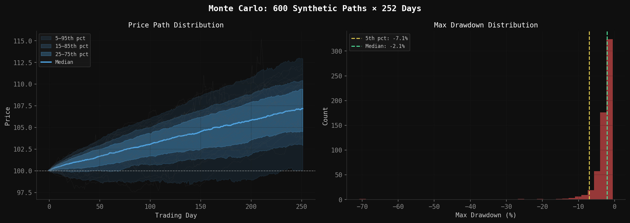
A single synthetic path is an anecdote. A thousand paths is a distribution.
Monte Carlo simulation runs the same generator with different seeds and collects the resulting strategy performance metrics. The output is a distribution over possible outcomes—not a single number—which is far more useful for risk assessment.
def monte_carlo_paths(
    n_paths: int = 1000,
    T: int = 252,
    S0: float = 100.0,
    generator_kwargs: dict = None,
    seed_start: int = 0,
) -> pd.DataFrame:
    """
    Run n_paths independent synthetic simulations.
    Returns DataFrame with one column per path (prices, indexed by day).
    """
    if generator_kwargs is None:
        generator_kwargs = {}

    gen = SyntheticMarketGenerator(**generator_kwargs)
    all_prices = np.zeros((T, n_paths))

    for i in range(n_paths):
        df = gen.generate(T=T, S0=S0, seed=seed_start + i)
        all_prices[:, i] = df['price'].values

    return pd.DataFrame(all_prices, columns=[f'path_{i}' for i in range(n_paths)])


def summarize_monte_carlo(paths_df: pd.DataFrame, S0: float = 100.0) -> dict:
    """
    Compute summary statistics across all Monte Carlo paths.
    """
    final_prices = paths_df.iloc[-1]
    final_returns = final_prices / S0 - 1

    # Per-path max drawdown
    max_drawdowns = []
    for col in paths_df.columns:
        prices = paths_df[col]
        dd = ((prices / prices.cummax()) - 1).min()
        max_drawdowns.append(dd)
    max_drawdowns = np.array(max_drawdowns)

    results = {
        'mean_return':       final_returns.mean(),
        'median_return':     final_returns.median(),
        'std_return':        final_returns.std(),
        'pct5_return':       final_returns.quantile(0.05),
        'pct95_return':      final_returns.quantile(0.95),
        'prob_positive':     (final_returns > 0).mean(),
        'mean_max_dd':       max_drawdowns.mean(),
        'median_max_dd':     np.median(max_drawdowns),
        'worst_max_dd':      max_drawdowns.min(),
        'pct5_max_dd':       np.percentile(max_drawdowns, 5),
    }

    print(f"\nMonte Carlo Summary ({len(paths_df.columns)} paths, {len(paths_df)} days)")
    print("─" * 50)
    print(f"{'Mean annual return':<28} {results['mean_return'] * 100:>8.1f}%")
    print(f"{'5th pct return':<28} {results['pct5_return'] * 100:>8.1f}%")
    print(f"{'95th pct return':<28} {results['pct95_return'] * 100:>8.1f}%")
    print(f"{'Prob(positive return)':<28} {results['prob_positive'] * 100:>8.1f}%")
    print(f"{'Mean max drawdown':<28} {results['mean_max_dd'] * 100:>8.1f}%")
    print(f"{'Worst max drawdown':<28} {results['worst_max_dd'] * 100:>8.1f}%")
    print(f"{'5th pct max drawdown':<28} {results['pct5_max_dd'] * 100:>8.1f}%")

    return results


# Example: run 500 paths and summarize
paths = monte_carlo_paths(n_paths=500, T=252, S0=450.0, seed_start=1000)
summary = summarize_monte_carlo(paths, S0=450.0)
11. What Synthetic Data Cannot Do
This is the part that deserves more space than it usually gets.
It doesn’t model economic causation. Real markets move on Fed announcements, earnings surprises, geopolitical shocks, credit events. A stochastic model has no knowledge of any of this. It can reproduce the statistical shape of volatility clustering without knowing why volatility clusters. This matters because the causal mechanisms that create market dynamics in the future may differ systematically from those that created them in the past.
Correlation structure breaks in crises. During normal markets, equity-bond correlations are reliably negative (~-0.4). During some crisis periods, both equities and bonds sell off simultaneously (as in 2022). A fixed correlation matrix misses this regime-dependence entirely. You can partially address this with regime-conditional correlations, but it adds significant complexity.
The tails are still underestimated. Even with Student’s t at ν = 4.51, the synthetic model underestimates the frequency of truly extreme events. The 1987 Black Monday crash was a 22% single-day decline—an event that would occur essentially never even under our fat-tailed model. The generator calibrates to the statistical distribution of historical returns, but the most extreme events are by definition underrepresented in any finite historical sample.
It is dangerous as training data. I covered this in the old post, but it bears repeating. Training a model on synthetic data risks teaching it to recognize patterns that exist in the simulator’s assumptions rather than in real market structure. The model can overfit to your stochastic model’s quirks. Use synthetic data to test robustness; be extremely cautious about using it to train signal models.
It says nothing about structural regime changes. The Markov transition matrix was estimated from 1993–2025 data. If we enter a genuinely new macroeconomic regime—say, structurally higher inflation, or a period of elevated geopolitical fragmentation that disconnects global markets—those transition probabilities are wrong. The model doesn’t know what it doesn’t know.
Despite all of this, the tool is genuinely useful. The failure modes it surfaces are real failure modes—they just tend to be different failure modes than the ones historical data surfaces. That difference is exactly the point.
12. A Complete Worked Example
Putting it all together in a single callable pipeline:
import numpy as np
import pandas as pd
from scipy import stats


def run_full_synthetic_analysis(
    scenarios: list[str] = None,
    n_monte_carlo: int = 500,
    T: int = 252,
    S0: float = 100.0,
    seed: int = 42,
) -> dict:
    """
    Run the full synthetic market analysis pipeline:
    1. Generate base calibration path
    2. Run Monte Carlo over base parameters
    3. Generate all requested scenarios
    4. Report summary statistics for each

    Returns dict of scenario_name -> summary stats.
    """
    if scenarios is None:
        scenarios = ['crash', 'choppy', 'stagflation', 'bull', 'slow_bleed',
                     'flash_crash', 'sideways', 'bear']

    results = {}

    print("=" * 70)
    print("Synthetic Market Analysis")
    print("=" * 70)

    # Base calibration
    gen = SyntheticMarketGenerator()
    base_df = gen.generate(T=T, S0=S0, seed=seed)
    base_return = base_df['price'].iloc[-1] / S0 - 1
    base_mdd = ((base_df['price'] / base_df['price'].cummax()) - 1).min()

    print(f"\nBase generator (1 path, {T} days):")
    print(f"  Return:       {base_return * 100:>7.1f}%")
    print(f"  Max Drawdown: {base_mdd * 100:>7.1f}%")

    # Monte Carlo on base
    print(f"\nRunning {n_monte_carlo} Monte Carlo paths...")
    paths = monte_carlo_paths(n_paths=n_monte_carlo, T=T, S0=S0, seed_start=1000)
    mc_summary = summarize_monte_carlo(paths, S0=S0)
    results['base_monte_carlo'] = mc_summary

    # Scenario runs
    print("\n" + "─" * 70)
    print(f"\n{'Scenario':<16} {'Return':>10} {'Sharpe':>10} {'Max DD':>10}")
    print("─" * 50)

    for scenario_name in scenarios:
        try:
            df = generate_scenario(scenario_name, T=T, S0=S0, seed=seed)
            log_rets = np.log(df['price'] / df['price'].shift(1)).dropna()
            ret = df['price'].iloc[-1] / S0 - 1
            mdd = ((df['price'] / df['price'].cummax()) - 1).min()
            ann_vol = log_rets.std() * np.sqrt(252)
            ann_ret = log_rets.mean() * 252
            sharpe = ann_ret / ann_vol if ann_vol > 0 else 0

            print(f"{scenario_name:<16} {ret * 100:>9.1f}% {sharpe:>10.2f} {mdd * 100:>9.1f}%")
            results[scenario_name] = {
                'return': ret, 'sharpe': sharpe, 'max_drawdown': mdd,
                'annual_vol': ann_vol,
            }
        except Exception as e:
            print(f"{scenario_name:<16} ERROR: {e}")

    print("\n" + "=" * 70)
    return results


# Run it
if __name__ == '__main__':
    all_results = run_full_synthetic_analysis(
        n_monte_carlo=500,
        T=252,
        S0=450.0,
        seed=42,
    )
13. Key Takeaways
The goal of a synthetic market generator is not to predict the future. It is to build a machine for asking what if—with enough statistical discipline that the answers carry real information.
A few things I’ve learned from building and using this:
Layer complexity incrementally. GBM first, then GARCH, then fat tails, then regime switching. Each layer should be validated against data before adding the next. If you add everything at once, you have no idea which component is producing which effect. This becomes super duper important, especially when you are trying to figure out whether the Sharpe of 3.0 is real with ROI of 8000%.
Match moments, not prices. The generator should reproduce annualized return, volatility, skewness, excess kurtosis, lag-1 autocorrelation, and volatility clustering. These are the moments that matter for strategy behavior. The specific prices are irrelevant.
Regime transitions are the most important calibration input. Getting the transition matrix right — especially the crisis regime’s diagonal (how sticky crashes are)—has more impact on strategy stress-test results than almost any other parameter choice.
Run enough paths. Single synthetic paths are anecdotes. The minimum useful Monte Carlo run is probably 250–500 paths for stable statistics on tail metrics. Max drawdown in particular has high variance in finite samples.
Validate against the source. Always run KS tests and visual diagnostics comparing synthetic returns to the historical returns used for calibration. If the synthetic distribution is statistically distinguishable from the real distribution (p < 0.05), the calibration is wrong.
And finally: synthetic markets surface failure modes that history cannot. I mean that is the entire point. The scenario that breaks your strategy is almost never the scenario you expected, and almost always the one you didn’t have data for.
14. Python Code
I’ve shared all the code on this GitHub repo here:
Generates realistic synthetic financial price paths by combining five statistical models:
GBM — geometric Brownian motion baseline
GARCH(1,1) — volatility clustering (persistence after shocks)
Student’s t — fat tails (4× more extreme events than Gaussian)
Ornstein-Uhlenbeck — mean reversion in returns and VIX
Markov regime switching — Bull / Bear / Crisis / Choppy regimes with calibrated transition probabilities
Calibrated to 30+ years of SPY data (1993–2025).
All code is open source — use it, modify it, build on it. No guarantees about correctness or performance. Test everything yourself before deploying with real capital.
Remember: Alpha is never guaranteed. And the backtest is a liar until proven otherwise. And could be a liar even with fake synthetic data.
The material presented in Math & Markets is for informational purposes only. It does not constitute investment or financial advice. This analysis probably contains errors — if you find them, let me know.
Great article! i think forms of bootstrap offer more potential when selected properly but I havent done any real testing of this. Section 8.3 is a great insight! keep it coming...
Question, would Monte Carlo simulations solve the same problem?