
Stress-Testing V6 with Synthetic Markets (Part 1: Building the Stochastic Model)
Part 52 is about extending the synthetic data testing and building stochastic models

This is part 52 of my series — Building & Scaling Algorithmic Trading Strategies
The V6 Dual Allocator has come a long way since Part 1, where this whole series started with a simple moving average strategy and a question: can I build something that reacts to trends without predicting the future?
Fifty parts later, the strategy has survived the lookahead bias massacre (Part 32 rebuild), an attempt to push Sharpe above 1.0 with options overlays (Part 39), rigorous parameter optimization (Part 48), plus experiments with ML regime classification, end-of-day execution filters, and volatility gates.
But all of that was historical backtesting on data from 2015–2025, which means V6 has seen exactly one flash crash (COVID), one sustained bear market (2022), and zero prolonged stagflation periods. After running the synthetic training experiment with the hybrid ensemble, I couldn’t stop wondering: should I actually trust V6 against markets that haven’t happened yet?
So I built a synthetic market generator calibrated to 32 years of SPY data, with the goal of stress-testing V6 against eight distinct scenarios to find the failure modes and see if the strategy’s core design actually holds up. Part 1 covers the math behind the generator, and Part 2 will cover the V6 results.
1. Why Synthetic Testing?
V6 relies on three core mechanisms: VIX regime detection to distinguish calm from chaotic markets, a 20-day moving average velocity signal for momentum, and position switching between TQQQ, QQQ, TLT, and cash depending on what the signals say.
Each of these mechanisms was tuned on historical data, and that’s a problem. The 2015–2025 window gave me exactly one of each major market event, so V6 may simply be overfit to those specific patterns. Synthetic testing lets me ask what happens if we get a different kind of crash—one that recovers faster, or slower, or not at all.
2. Calibrating to Real SPY
Before generating fake markets, I needed to understand what real markets actually look like, so I analyzed 32 years of SPY data from 1993–2025 and extracted the key statistical properties that any realistic synthetic generator needs to reproduce.
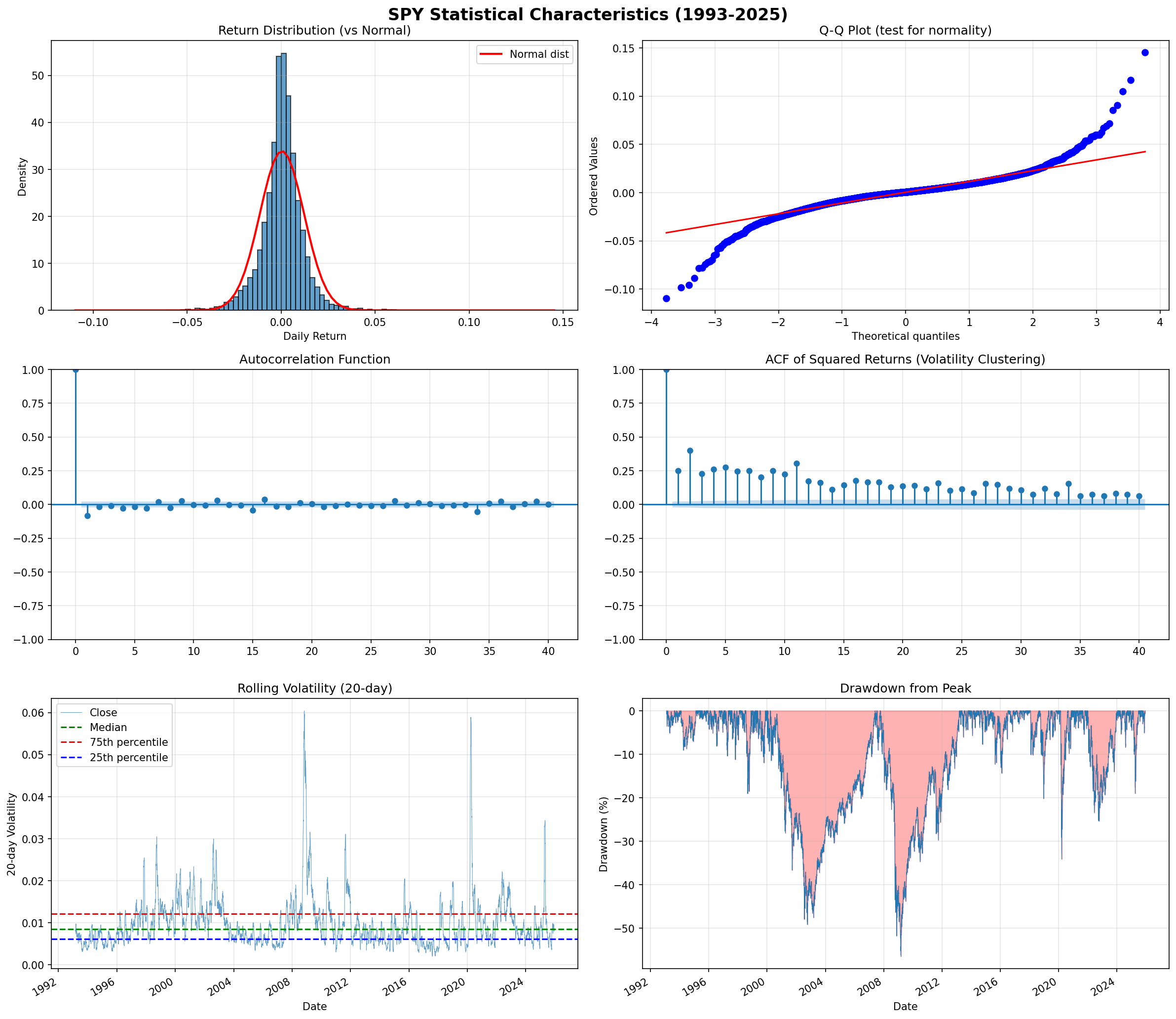
2.1 Returns and Volatility
The baseline numbers are straightforward: SPY has delivered about 10.13% annual returns with 18.68% volatility, giving a Sharpe ratio around 0.542. These become the central parameters for the generator—any synthetic scenario should orbit around these values unless I’m explicitly stress-testing an extreme environment.
2.2 Fat Tails
This is where it gets interesting. SPY has an excess kurtosis of 11.72, which sounds like an obscure statistical footnote until you realize what it means in practice. A normal distribution has excess kurtosis of zero, so 11.72 means extreme events occur roughly 4× more frequently than a Gaussian model would predict.
Kurtosis = E[(X - μ)⁴] / σ⁴ - 3 = 11.72Under normality, a 3-sigma move should happen about 0.27% of the time. With SPY’s fat tails, it happens closer to 1.2% of the time. This is why market crashes feel “unexpected”—our intuitions are calibrated to thinner tails than reality actually delivers.
2.3 Volatility Clustering
High volatility tends to beget more high volatility. The autocorrelation of squared returns (a standard proxy for volatility persistence) comes in at 0.248 at lag-1, which means knowing today’s volatility tells you something meaningful about tomorrow’s. This effect persists for 5–20 trading days, explaining why VIX spikes tend to cluster rather than appear in isolation.
2.4 Regime Distribution
I classified each historical day into one of four regimes based on returns and volatility:
Regime     Frequency    Characteristics
─────────────────────────────────────────────────────
Bull       48.3%        Positive returns, low vol
Bear       19.5%        Negative returns, elevated vol
Crisis      6.2%        Extreme negative returns, vol spike
Choppy      3.8%        High vol, no clear direction
The remaining ~22% falls into “normal” or transitional periods. These frequencies become the transition probabilities in the regime-switching component of the model.
3. The Stochastic Model Stack
No single model captures all of SPY’s statistical properties, so I built six separate models and combined them into a single generator.
3.1 Geometric Brownian Motion (GBM)
GBM serves as the baseline, where returns follow the classic stochastic differential equation:
dS = μS dt + σS dWHere μ is drift (10.13% annualized), σ is volatility (18.68%), and dW is a Wiener process. GBM is elegant but fundamentally wrong—it assumes constant volatility and Gaussian returns, neither of which matches reality. Still, it provides the skeleton that everything else builds on.
3.2 GARCH(1,1) for Volatility Clustering
To capture the persistence in volatility that the ACF revealed, I layer on a GARCH model:
σₜ² = ω + α·εₜ₋₁² + β·σₜ₋₁²The parameters α = 0.09 and β = 0.89 were estimated from SPY’s historical returns, and their sum of 0.98 (close to 1) indicates high persistence. After a volatility spike, it takes weeks to decay back to baseline—exactly what we observe in real markets.
3.3 Student’s t for Fat Tails
Instead of drawing the noise term dW from a normal distribution, I use a Student’s t distribution with degrees of freedom calibrated to match SPY’s kurtosis:
ν = 6 / (excess kurtosis) + 4 ≈ 4.5Lower degrees of freedom means fatter tails, and at ν = 4.5, the distribution produces roughly 4× more extreme events than a Gaussian would—matching what we see in the actual data.
3.4 Mean Reversion
SPY shows slight negative autocorrelation at lag-1 (about -0.08), meaning large up days tend to be followed by modest pullbacks and vice versa. I add an Ornstein-Uhlenbeck term to capture this:
dX = θ(μ - X) dt + σ dWThe parameter θ controls mean-reversion speed, and including this prevents the model from generating unrealistic straight-line trends that would never occur in actual markets.
3.5 Regime-Switching Markov Model
The four regimes (bull, bear, crisis, choppy) each have their own return and volatility parameters, with transitions governed by a Markov chain whose probabilities were estimated from the historical data:
From/To      Bull    Bear    Crisis    Choppy
───────────────────────────────────────────────
Bull         0.95    0.03    0.01      0.01
Bear         0.10    0.85    0.03      0.02
Crisis       0.15    0.25    0.55      0.05
Choppy       0.20    0.15    0.05      0.60
The diagonal dominance reflects regime persistence—once you’re in a bear market, you tend to stay there for a while. But crises are inherently unstable and transition out quickly, either to recovery or to a deeper bear phase.
3.6 The Combined Model
The final generator brings all of this together in a specific sequence: draw the current regime from the Markov chain, set drift and volatility from that regime’s parameters, apply the GARCH update to volatility, draw the return shock from the Student’s t distribution, add the mean-reversion adjustment, and finally compute the price change via GBM dynamics. The result is synthetic SPY paths with realistic fat tails, volatility clustering, and regime structure.
4. Generating Correlated Assets
V6 trades four assets—SPY (as a proxy for QQQ), TQQQ, TLT, and cash—so the synthetic generator needs to produce all four with realistic correlations between them.
4.1 TQQQ
TQQQ is 3× leveraged QQQ with daily rebalancing, so the return relationship is:
r_TQQQ = 3 × r_QQQ - decayThe decay term (roughly 0.03% daily) captures the volatility drag that comes from daily rebalancing. In choppy markets, this drag means TQQQ can actually lose value even when QQQ ends up flat—a critical dynamic for any strategy that uses leveraged ETFs.
4.2 TLT
Bonds typically move inversely to equities during stress, which is the whole reason V6 uses TLT as a hedge. I model TLT with a -0.4 correlation to SPY (estimated from historical data), 4% annual drift reflecting long-run Treasury returns, and 15% annual volatility. The negative correlation is what makes TLT valuable during equity crashes—exactly what V6 relies on when VIX exceeds 30.
4.3 VIX
VIX is mean-reverting around 18 under normal conditions, but spikes sharply during equity drawdowns:
dVIX = κ(V̄ - VIX) dt + σ_VIX dW + jumpThe jump term fires whenever SPY’s daily return is worse than -2%, which captures the fundamental asymmetry in volatility behavior: VIX drifts slowly downward in calm markets but spikes instantly when things go wrong.
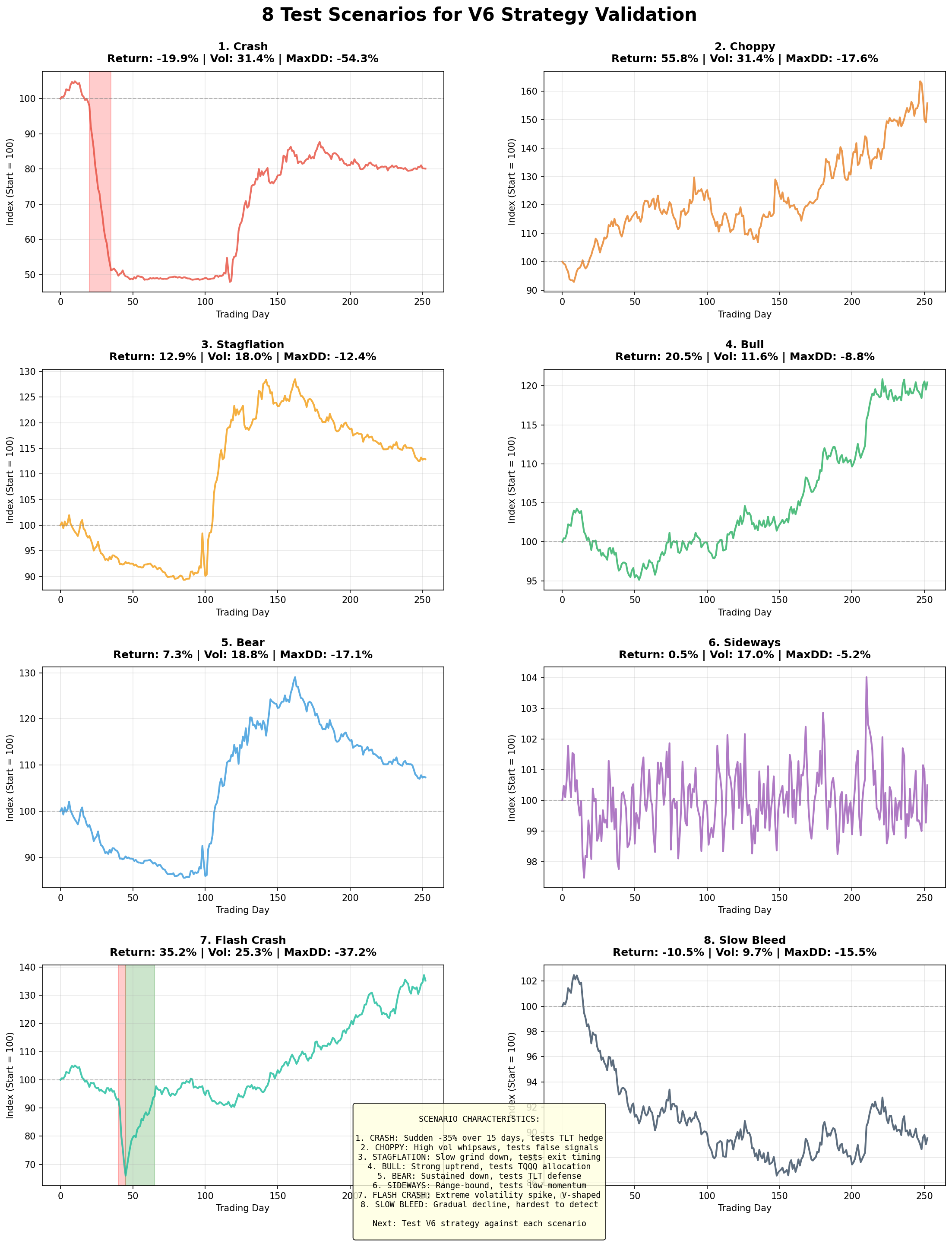
5. The Eight Scenarios
With the generator built, I defined eight stress-test scenarios designed to probe different aspects of V6’s behavior:
Scenario       Description                      Key Parameter Tweaks
────────────────────────────────────────────────────────────────────────────
Crash          Sudden -35% drawdown, recovery   Crisis regime for 40 days
Choppy         High volatility, no trend        Vol = 35%, drift = 0%
Stagflation    Slow grind down                  Drift = -8%, vol = 15%
Bull           Sustained uptrend                Drift = 20%, vol = 12%
Bear           Sustained downtrend              Drift = -15%, vol = 25%
Sideways       Range-bound                      Drift = 0%, vol = 10%, high mean-reversion
Flash Crash    V-shaped crash + rapid recovery  -37% in 10 days, full recovery in 20
Slow Bleed     Gradual decline, low vol         Drift = -10.5%, vol = 12%
Each scenario runs for 252 trading days (one year), and the generator produces complete SPY, TQQQ, TLT, and VIX paths that V6 then trades against.
6. What’s Next
Part 2 covers the results: where V6 excels, where it fails, and what those failure modes reveal about the strategy’s underlying design. The spoiler is that the core design is sound, but two scenarios exposed critical weaknesses that would never show up in a standard historical backtest.
Remember: Alpha is never guaranteed. And the backtest is a liar until proven otherwise.
Options and derivatives are complex instruments and not suitable for all investors. This analysis probably contains errors — if you find them, let me know.
The material presented in Math & Markets is for informational purposes only. It does not constitute investment or financial advice.