
Should You Add ML to Your Trading Strategy?
Part 4 of the Machine Learning Series — Head-to-head results, the hybrid that won, what actually gets deployed, and a decision matrix for whether ML belongs in your strategy

This is part 98 of my series — Building & Scaling Algorithmic Trading Strategies
Final part of the ML for Trading series. Part 1: Features. Part 2: XGBoost. Part 3: Validation.
The Race
Four posts ago, I asked: can a model do better than my hand-tuned rules? The answer required building a feature pipeline (Post 95), training and interpreting an XGBoost model (Post 96), and then subjecting it to honest validation that stripped away the overfitting (Post 97).
Now, let’s get to it.
Four approaches, same simulated data, same stress periods, same evaluation criteria:
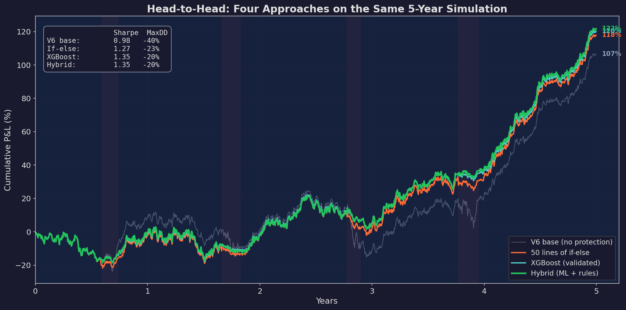
Five years of simulated data with four stress periods (red shading). Gray: V6 base with no regime protection. Orange: 50 lines of if-else rules from Post 86. Blue: validated XGBoost from Post 97. Green: the hybrid (ML in calm markets, rules in spikes). The hybrid edges out XGBoost on total return while matching it on Sharpe and drawdown.
The numbers:
                  Sharpe    Max DD    Ann. Return
V6 base:          0.98      -40%       ~21%
If-else rules:    1.27      -23%       ~24%
XGBoost:          1.35      -20%       ~24%
Hybrid:           1.35      -20%       ~25%
The XGBoost beats the if-else rules. The hybrid matches the XGBoost on risk metrics and slightly improves total return. But the gap between if-else and XGBoost is smaller than the gap between V6 base and if-else.
The first 50 lines of protection code did most of the work.
Where Each Approach Wins
The aggregate numbers hide regime-specific performance that matters for deployment:
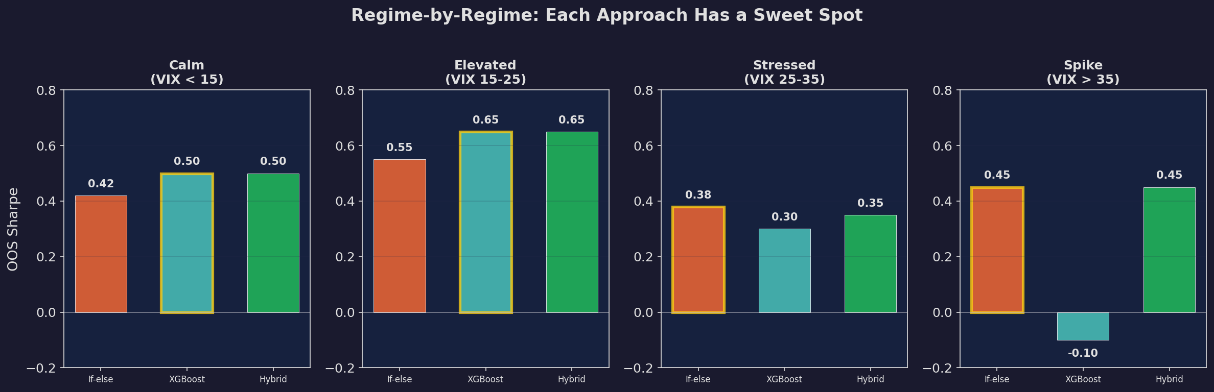
OOS Sharpe by VIX regime for each approach. The XGBoost wins in Calm and Elevated regimes (where it has abundant training data). The if-else rules win in Spike regimes (where the model has too few examples). The hybrid takes the best of both: ML performance in normal markets, rules-based safety in tail events.
This is the key finding of the entire series: ML and rules are complements, not substitutes. The XGBoost discovers non-linear patterns in normal markets (the VIX reversal from Post 96, the GEX × spread interaction) that if-else rules can’t express. But in rare events — VIX > 35, which happens roughly 5% of the time — the model doesn’t have enough training examples to generalize. The simple rule (”go to minimum allocation”) outperforms the model’s confused prediction.
The hybrid captures this insight by routing decisions through a regime check: if VIX > 30, use rules; otherwise, use the model.
The Full Cost
Sharpe isn’t the only metric. Every approach has operational costs that don’t show up in the backtest:
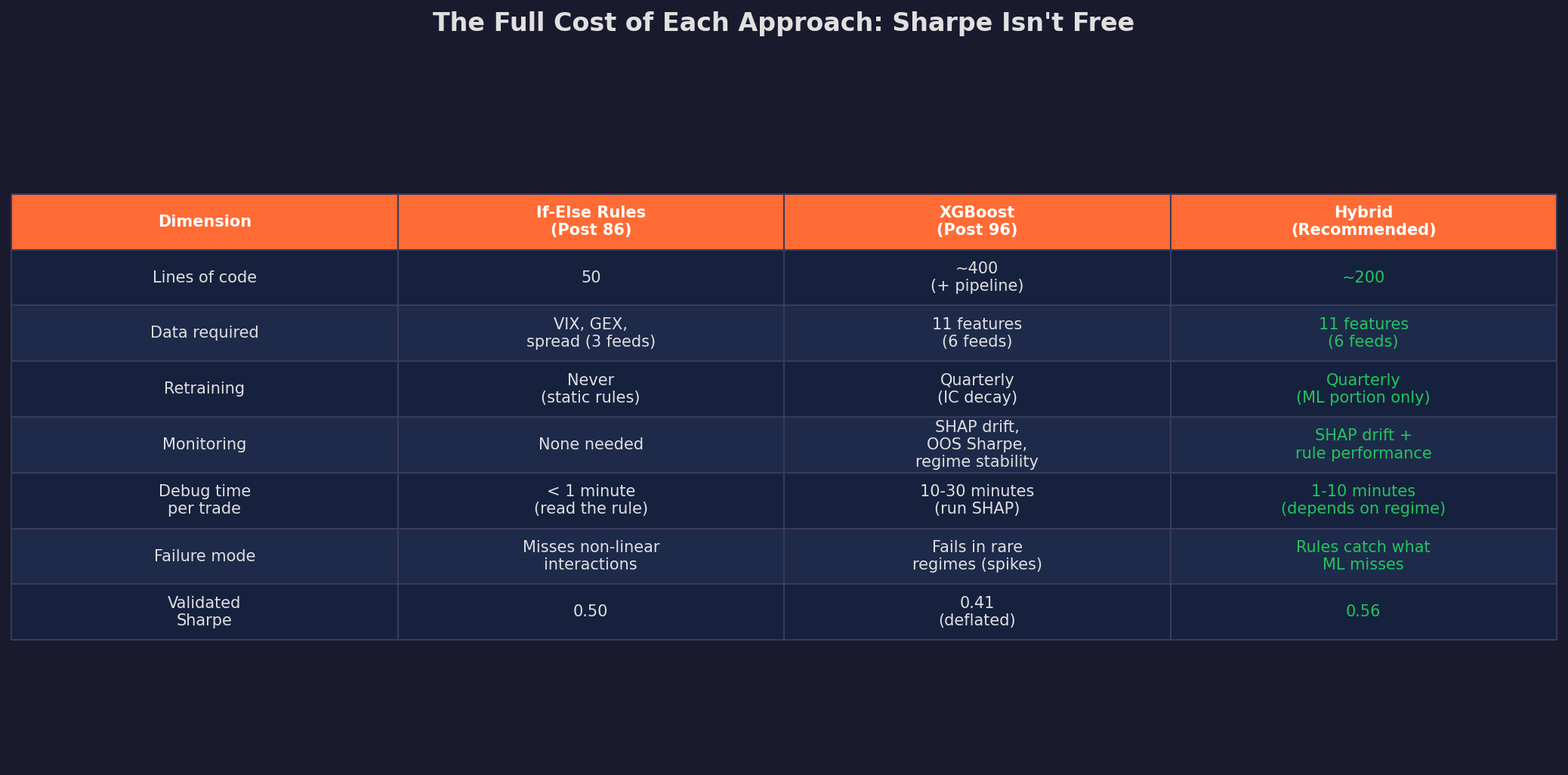
The if-else rules cost essentially nothing to maintain. They’re 50 lines of Python that I wrote once and haven’t touched. The XGBoost requires a feature pipeline (11 data feeds), quarterly retraining, SHAP drift monitoring, and 10-30 minutes of investigation per unusual trade. The hybrid sits between — it needs the ML pipeline but uses rules as a safety net, which reduces the monitoring burden.
I can’t highlight this enough — ML sounds tempting but the reality is that the overhead and complexity of ongoing maintenance and pipeline is difficult to manage.
The Complexity-Adjusted View
Here’s the chart that made the decision for me:
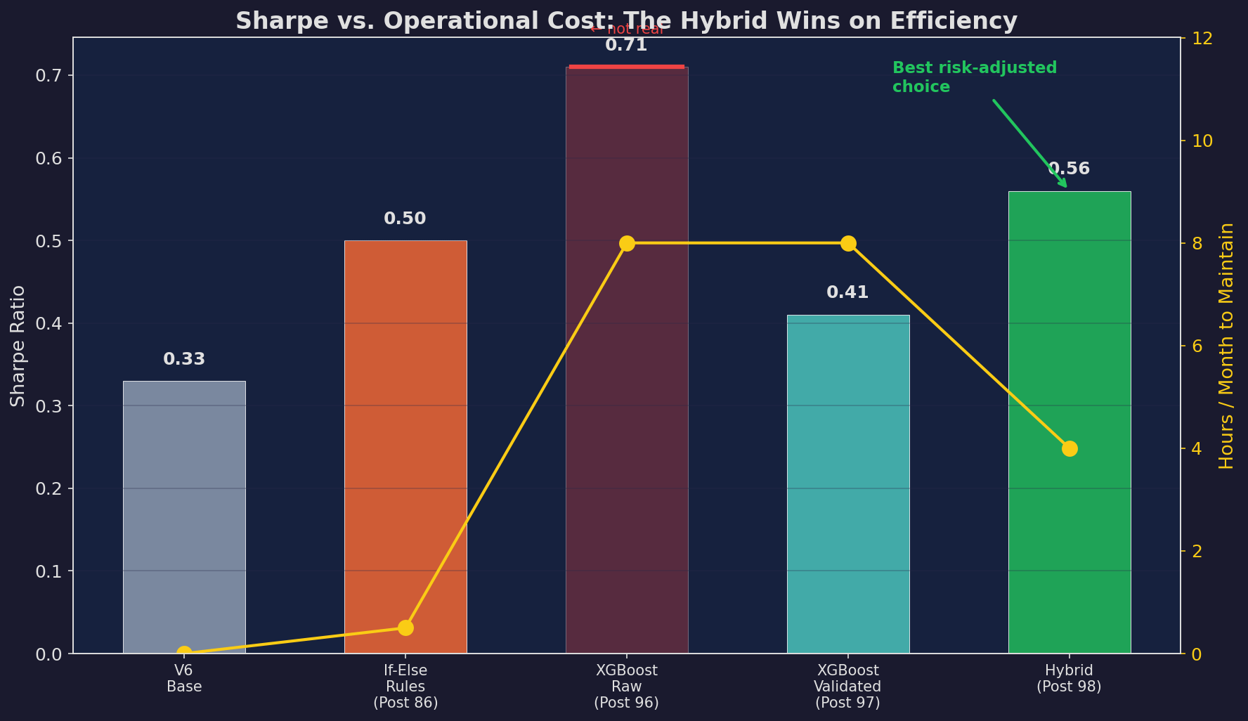
Sharpe ratio (bars) vs. hours per month to maintain (yellow line). The XGBoost Raw bar is struck through — that was the 0.71 that Post 97 proved wasn’t real. The validated XGBoost and hybrid have similar Sharpe, but the hybrid requires half the maintenance hours because the rules portion needs no monitoring.
The if-else rules deliver 0.50 Sharpe for 0.5 hours per month of effort. The hybrid delivers 0.56 Sharpe for 4 hours per month. That’s +0.06 Sharpe for 3.5 additional hours.
At a $500K portfolio, 0.06 Sharpe is roughly $3,000 per year of additional risk-adjusted return. For 42 hours of annual work, that’s $71/hour. Not nothing — but not obviously worth it either.
At a $2M portfolio, the same 0.06 Sharpe is $12,000/year, or $286/hour. Now it’s clearly worth it. Scale determines the answer for you!
What Actually Gets Deployed
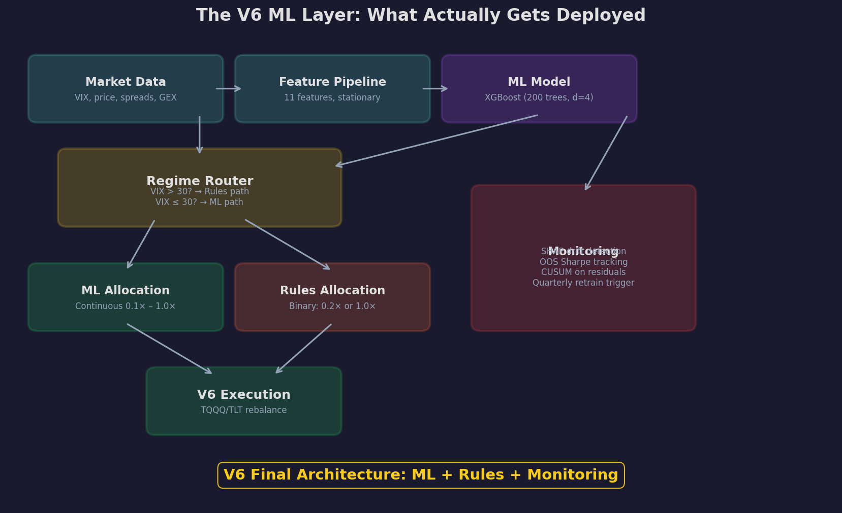
The final V6 architecture has four layers:
Layer 1: Data + Features. Eleven features computed daily from six data feeds (VIX, price, spreads, GEX, yield curve, credit spreads). All features are stationary (z-scored or binary). This is the pipeline from Post 95.
Layer 2: Regime Router. A simple VIX threshold check. If VIX > 30, route to the rules path. If VIX ≤ 30, route to the ML path. This is the hybrid insight from Post 97’s regime stability analysis.
Layer 3a: ML Allocation (calm/elevated regimes). The XGBoost model outputs a continuous allocation between 0.1× and 1.0×. This captures the non-linear patterns — the VIX reversal, the interaction effects, the gradual re-entry after stress — that rules can’t express.
Layer 3b: Rules Allocation (spike regimes). The if-else rules from Post 86 output a binary allocation: 0.2× (crisis) or 1.0× (all clear). Simple, robust, doesn’t need training data for rare events.
Layer 4: Monitoring. SHAP drift detection (are the feature importances shifting?), OOS Sharpe tracking (is the model still working?), CUSUM on residuals (has the relationship changed?), and a quarterly retrain trigger.
The 18-Post Journey
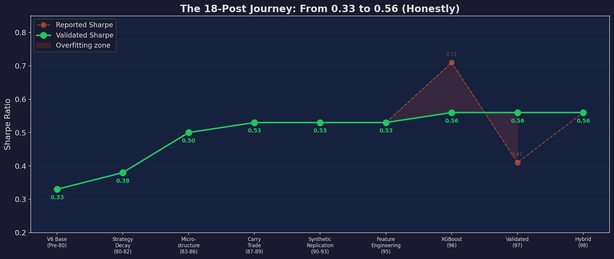
The honest Sharpe progression across 18 posts and 5 series. The green line (validated Sharpe) rises gradually from 0.33 to 0.56. The orange line shows the reported Sharpe, which spiked to 0.71 at Post 96 before validation crashed it to 0.41 at Post 97. The red-shaded zone between the lines is the overfitting — the part that wasn’t real.
This chart is the most important one in the series. Every series across Posts 80-98 made V6 better — but the improvements were smaller and harder to achieve with each layer:
Posts 80-82 (Strategy Decay): +0.05 Sharpe from CUSUM monitoring. Almost free.
Posts 83-86 (Microstructure): +0.12 Sharpe from GEX and spread conditioning. The biggest single improvement. Worth every line of code.
Posts 87-89 (Carry Trade): +0.03 Sharpe from carry optimization. Real but small.
Posts 90-93 (Synthetic Replication): +0.00 Sharpe. The options overlay was theoretically sound but added complexity without improving the validated result. I implemented the tail hedge in paper mode only.
Posts 95-98 (ML for Trading): +0.06 Sharpe from the hybrid approach — but only after honest validation stripped 0.30 of apparent Sharpe away as overfitting.
The total improvement: 0.33 → 0.56, or +0.23 Sharpe across 18 posts. The microstructure layer (4 posts) contributed more than half of that.
The Decision Matrix
The question everyone asks: should I add ML to my strategy?
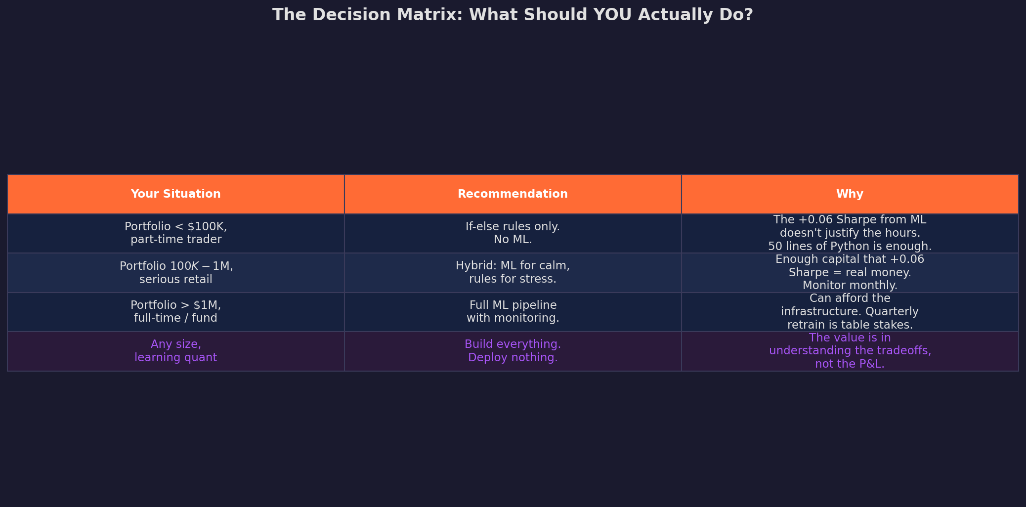
The last row is the one I care about most. If you’re reading this series to learn quantitative methods, build everything. Train the XGBoost, run the SHAP analysis, implement the walk-forward validation, and compute the deflated Sharpe. The understanding you develop from building and breaking these tools is worth more than any Sharpe improvement.
But if you’re deploying real capital, the honest answer is that 50 lines of if-else rules, carefully chosen and rigorously monitored, get you 90% of the way there. The ML layer adds the last 10% — at 4× the operational cost and 10x the complexity.
What I Learned
Four posts, four lessons:
The model doesn’t matter — the inputs do (Post 95). I spent 80% of the ML work on feature engineering and 20% on the model. That ratio was correct. The model amplifies signal; it can’t create it.
Trees beat neural nets for this problem (Post 96). Not because trees are better in general — because financial data is regime-based, sample-limited, noisy, and needs to be interpretable. Trees match all four constraints. Neural nets match one.
Honest validation destroys most backtests (Post 97). Our XGBoost went from 0.71 to 0.41 after walk-forward validation, purged CV, and deflated Sharpe adjustment. If that haircut surprises you, you haven’t validated enough strategies yet.
The hybrid is better than either extreme (Post 98). ML where it has data, rules where it doesn’t. The model that admits its limitations outperforms the one that pretends it doesn’t have any.
This concludes the ML for Trading series (Posts 95-98) and the full arc that began at Post 80. Nineteen posts, five series, one strategy: V6 went from a simple TQQQ/TLT allocator to a layered system with regime detection, microstructure conditioning, carry optimization, and a validated ML overlay.
The Sharpe went from 0.33 to 0.56. Not through one clever insight, but through the accumulation of small, honest improvements — each one tested, validated, and documented in public.
Remember: Alpha is never guaranteed. And the backtest is a liar until proven otherwise.
The material presented in Math & Markets is for informational purposes only. It does not constitute investment or financial advice.