
When One Model Isn't Enough: Ensemble Regime Detection
Part 72 — HMM Series 3 of 3 — CUSUM, BOCPD, feature engineering, and the three-signal framework I'm testing for V6

This is part 72 of my series — Building & Scaling Algorithmic Trading Strategies
Parts 1 and 2 covered Hidden Markov Models: the theory, the algorithms, and the unavoidable detection lag. HMMs are the default tool for regime detection, but they’re not the only tool.
This post explores alternatives: changepoint detection methods, machine learning approaches, and ensemble techniques. I’ll also share what I’m currently evaluating for V6 — not a final decision, but a framework I’m testing because it’s practical and I can explain every component.
The goal isn’t to eliminate detection lag (we can’t) but to build a system that’s robust, interpretable, and doesn’t require a PhD to maintain.
Changepoint Detection: A Different Framing
HMMs model regimes as discrete states with transitions. Changepoint detection takes a different view: the data-generating process is stable until it suddenly shifts.
The question changes from “what state are we in?” to “did something just change?”
CUSUM (Cumulative Sum Control Charts)
CUSUM tracks cumulative deviations from an expected mean. When the cumulative deviation exceeds a threshold, a changepoint is signaled.
S⁺(t) = max(0, S⁺(t-1) + (r_t - μ₀) - k)
S⁻(t) = max(0, S⁻(t-1) - (r_t - μ₀) - k)

Signal changepoint when S⁺(t) > h or S⁻(t) > h

Where:
  μ₀ = expected mean under "normal" conditions
  k  = allowance parameter (slack before accumulating)
  h  = decision threshold
S⁺ detects upward shifts in mean; S⁻ detects downward shifts. The allowance k prevents small fluctuations from accumulating. The threshold h controls sensitivity vs. false alarms.
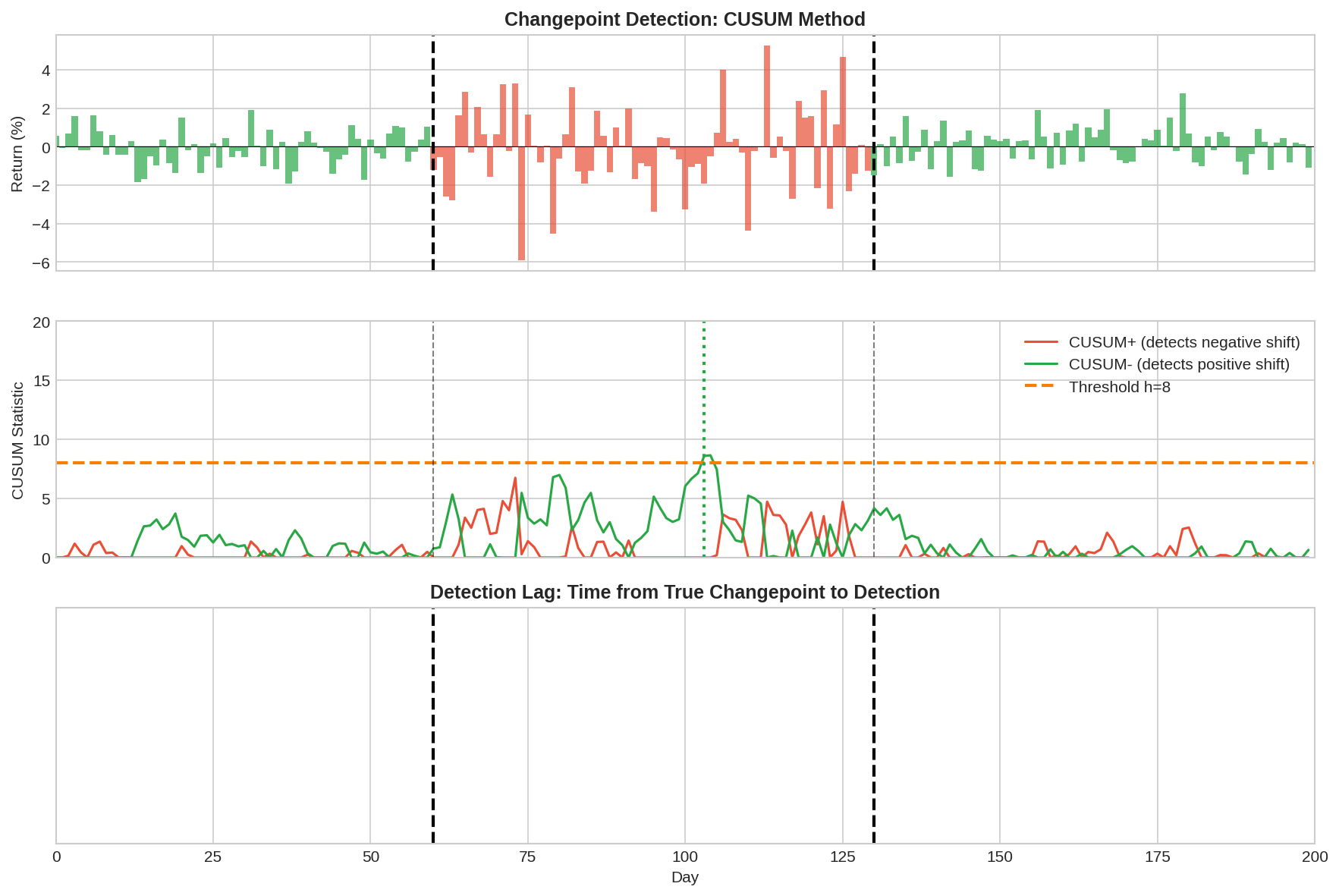
The middle panel shows the CUSUM statistics. Notice how S⁺ (red) accumulates during the bear market as negative returns pile up. When it crosses the threshold h=8, a changepoint is signaled.
Pros of CUSUM:
Simple and interpretable
Well-understood statistical properties
Easy to tune (just k and h)
Cons:
Assumes you know the “normal” mean μ₀
Threshold h trades off speed vs. false positives
Doesn’t give probability—just a binary signal
Bayesian Online Changepoint Detection (BOCPD)
BOCPD, introduced by Adams and MacKay (2007), is more sophisticated. It maintains a probability distribution over “run lengths” — how long since the last changepoint.
The intuition: at each time step, either we’re continuing the current regime (run length increases by 1) or a changepoint occurred (run length resets to 0). BOCPD computes the posterior probability of each possibility.
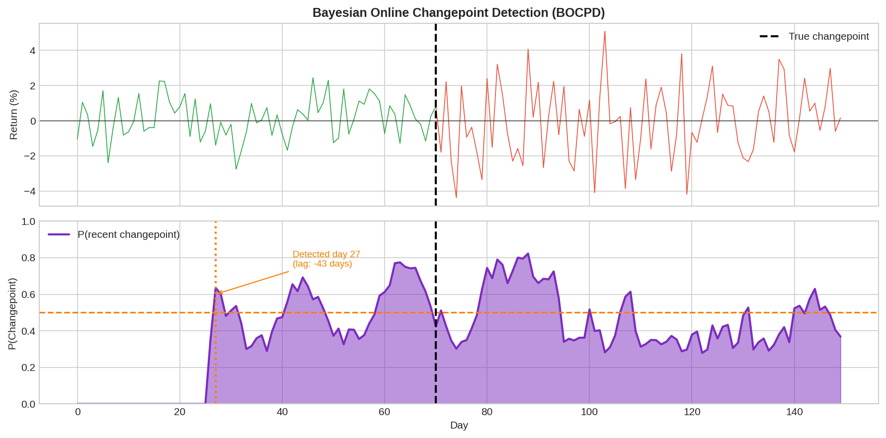
The bottom panel shows P(recent changepoint) — a continuous probability rather than a binary flag. This is more useful for sizing positions: you can reduce exposure proportionally as changepoint probability rises.
The BOCPD recursion:
P(r_t = 0 | data) ∝ H × Σ P(r_{t-1} | data) × P(x_t | r_{t-1})
P(r_t = r_{t-1}+1 | data) ∝ (1-H) × P(r_{t-1} | data) × P(x_t | r_{t-1})

Where:
  r_t     = run length at time t
  H       = hazard rate (prior probability of changepoint)
  P(x_t | r) = predictive probability of observation given run length
Pros of BOCPD:
Produces probabilities, not just flags
Naturally handles uncertainty
Can model different segment distributions
Cons:
More complex to implement
Requires specifying hazard rate and segment model
Still has detection lag (it’s Bayesian, not clairvoyant)
Machine Learning: Feature Engineering Matters More Than Algorithms
You can frame regime detection as a classification problem: given features, predict Bull or Bear. Random forests, gradient boosting, neural networks — all the usual suspects.
But here’s the thing: the features matter far more than the model.
A random forest with good features will crush a neural network with bad features. For regime detection, good features include:
Price-based:
  - Realized volatility (20-day, 60-day)
  - Return momentum (various lookbacks)
  - Drawdown from recent high
  - % of up days in lookback window

Volatility surface:
  - VIX level
  - VIX term structure (contango/backwardation)
  - VVIX (volatility of volatility)
  - Put/call skew

Credit/macro:
  - High yield spreads
  - Investment grade spreads
  - TED spread
  - Yield curve slope
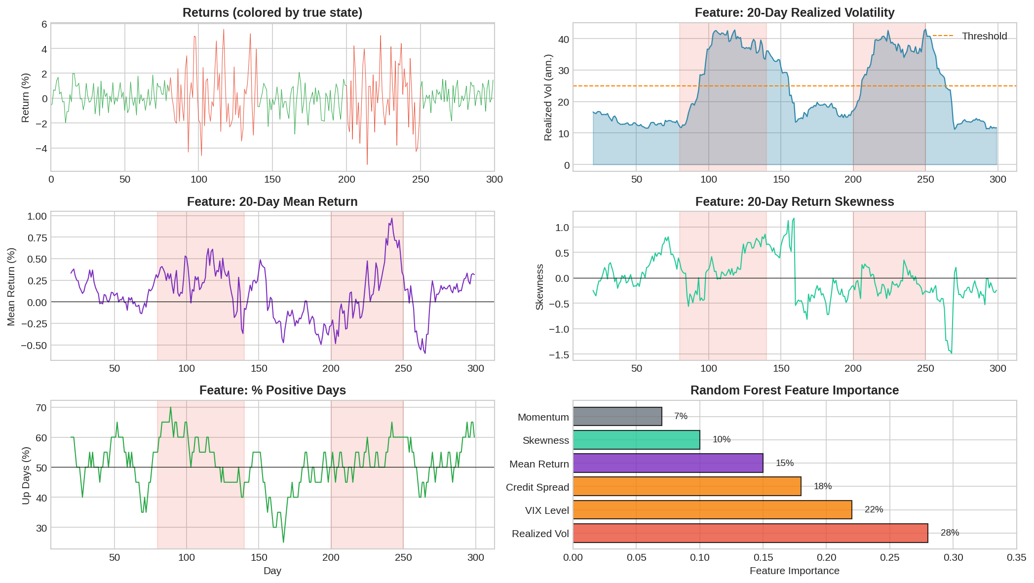
The chart shows several features and their behavior during bear regimes (shaded). Realized volatility is the single best feature — it reliably spikes during bear markets. But combining multiple features improves robustness.
Feature importance from a random forest trained on regime labels:
Feature             Importance
-----------------   ----------
Realized Vol        28%
VIX Level           22%
Credit Spread       18%
Mean Return         15%
Skewness            10%
Momentum             7%
Volatility dominates. This makes sense — bear markets are defined as much by volatility expansion as by negative returns.
The ML caveat:
Machine learning models are prone to overfitting, especially with regime data where you might only have a handful of bear markets in your training set. A model that perfectly classifies historical regimes may fail on the next one.
Mitigations:
Use simple models (random forest with few trees, logistic regression)
Regularize aggressively
Test on true out-of-sample periods (not random splits)
Prefer interpretable features over complex transformations
Ensemble Methods: Don’t Bet on One Signal
Single detectors fail in different ways:
HMM might lag during sharp crashes but handle gradual regime shifts well
VIX threshold is fast but noisy
CUSUM catches sustained shifts but misses brief spikes
Combining signals reduces reliance on any single method’s weaknesses.
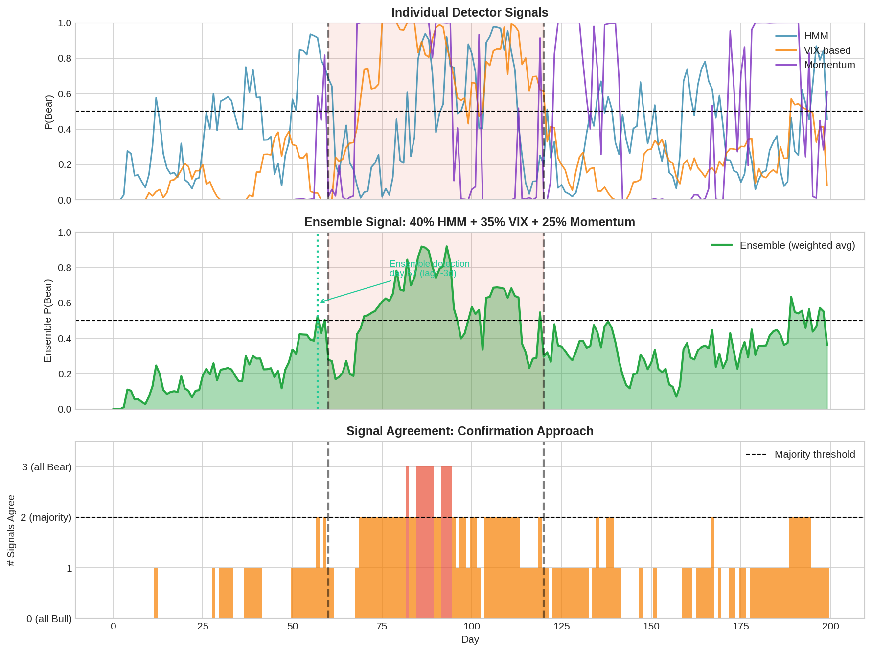
The top panel shows three individual signals: HMM, VIX-based, and momentum. Each has different timing and noise characteristics. The middle panel shows the ensemble (weighted average). The bottom panel shows signal agreement — how many detectors agree at each time.
Two ensemble approaches:
1. Weighted Average:
P(Bear)_ensemble = w₁ × P(Bear)_HMM + w₂ × P(Bear)_VIX + w₃ × P(Bear)_momentum

Example weights: 0.40, 0.35, 0.25
This gives a smooth probability that incorporates all signals. Tune weights based on historical performance or use equal weights as a baseline.
2. Confirmation (Majority Vote):
Signal Bear only if ≥2 of 3 detectors agree.

More conservative: require all 3 to agree.
More aggressive: require any 1 to trigger.
Confirmation reduces false positives but increases lag. You’re waiting for multiple signals to align.
Which is better? Depends on your cost function. If false positives are expensive (transaction costs, whipsaw), use confirmation. If lag is expensive (missing crash protection), use weighted average with lower threshold.
Comparing Methods
No method dominates on all dimensions:
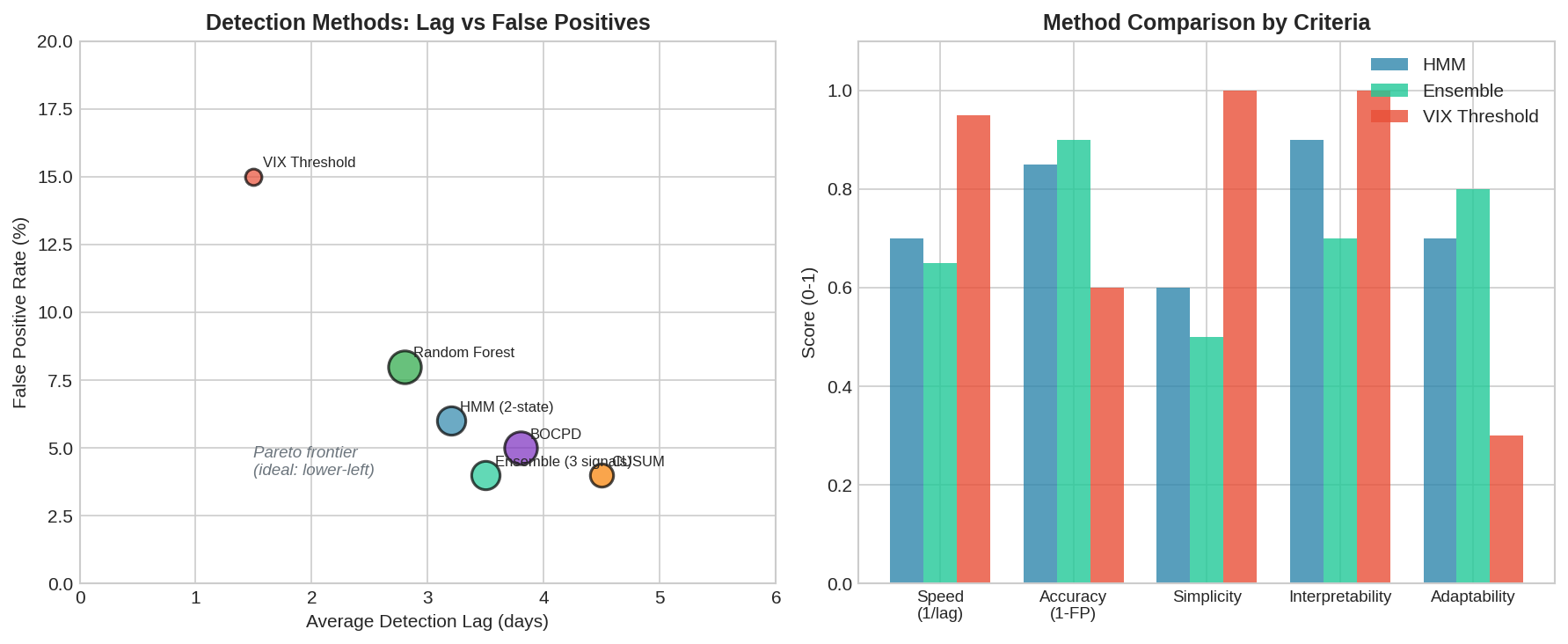
The left panel plots detection lag vs. false positive rate. Lower-left is better (fast and accurate), but no method lives there. You’re always trading off.
The right panel compares methods on multiple criteria:
Speed: How fast to detect (VIX threshold wins)
Accuracy: False positive rate (ensemble wins)
Simplicity: Ease of implementation (VIX threshold wins)
Interpretability: Can you explain decisions? (HMM, VIX win)
Adaptability: Handles novel regimes (ensemble, ML win)
My take: start simple, add complexity only if it helps.
A VIX threshold at 25 is dead simple and catches most bear markets within a day. It has high false positives, but you can filter with confirmation from a second signal. This beats a complex system you don’t understand.
What I’m Evaluating for V6
After all this analysis, here’s what I’m testing for potential integration into V6:
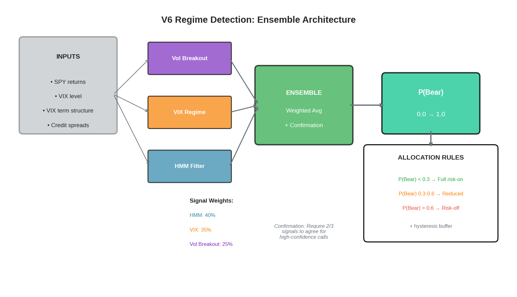
Three signal generators:
HMM Filter (40% weight)
2-state Gaussian HMM fitted on rolling 2-year window
Online filtering (forward algorithm only)
Outputs P(Bear) between 0 and 1
VIX Regime (35% weight)
Simple threshold logic with hysteresis
VIX < 18: P(Bear) = 0.1
VIX 18-25: P(Bear) = 0.3
VIX 25-35: P(Bear) = 0.6
VIX > 35: P(Bear) = 0.9
Volatility Breakout (25% weight)
20-day realized vol vs. 60-day baseline
If current vol > 1.5× baseline: P(Bear) = 0.7
Else: P(Bear) = 0.2
Ensemble aggregation:
P_bear = 0.40 * hmm_signal + 0.35 * vix_signal + 0.25 * vol_signal
Confirmation layer:
For high-confidence calls (P_bear > 0.7 or < 0.3), require at least 2/3 signals to agree
If signals disagree significantly, stay at neutral allocation
Allocation rules:
P(Bear) < 0.3    → Full risk-on (100% TQQQ)
P(Bear) 0.3-0.6  → Reduced exposure (50% TQQQ, 50% hedge)
P(Bear) > 0.6    → Risk-off (100% hedge)

Hysteresis: ±0.1 buffer to prevent thrashing
Why I’m testing this design:
Interpretable: I can explain every component. When the system signals Bear, I’ll know why.
Robust: No single signal failure kills the system. If HMM breaks, VIX and vol still work.
Tunable: Weights can be adjusted without rewriting code. Thresholds are explicit.
Testable: Each component can be backtested independently before committing to live use.
Implementation (Under Evaluation)
Core ensemble detector I’m testing:
"""
Ensemble Regime Detector - Under Evaluation for V6
Math & Markets - Post 71

All code is open source—use it, modify it, build on it.
No guarantees about correctness or performance.
Test everything yourself before deploying with real capital.

Author: K. Iyer
Substack: https://kniyer.substack.com
"""

import numpy as np

class EnsembleRegimeDetector:
    """
    Combines multiple regime signals into ensemble P(Bear).
    """

    def __init__(self, weights=None):
        """
        weights: dict with keys 'hmm', 'vix', 'vol'
        """
        self.weights = weights or {'hmm': 0.40, 'vix': 0.35, 'vol': 0.25}
        self.hmm_filter = None  # Initialize separately
        self.vol_baseline = None
        self.last_p_bear = 0.3  # For hysteresis

    def vix_signal(self, vix):
        """Convert VIX level to P(Bear)."""
        if vix < 18:
            return 0.1
        elif vix < 25:
            return 0.3
        elif vix < 35:
            return 0.6
        else:
            return 0.9

    def vol_signal(self, realized_vol, baseline_vol):
        """Compare current vol to baseline."""
        if baseline_vol <= 0:
            return 0.3

        ratio = realized_vol / baseline_vol
        if ratio > 1.5:
            return 0.7
        elif ratio > 1.2:
            return 0.4
        else:
            return 0.2

    def compute_ensemble(self, hmm_p_bear, vix, realized_vol, baseline_vol):
        """
        Compute weighted ensemble P(Bear).

        Returns: (p_bear, signals_dict, agreement)
        """
        # Individual signals
        p_hmm = hmm_p_bear
        p_vix = self.vix_signal(vix)
        p_vol = self.vol_signal(realized_vol, baseline_vol)

        signals = {'hmm': p_hmm, 'vix': p_vix, 'vol': p_vol}

        # Weighted average
        p_bear = (
            self.weights['hmm'] * p_hmm +
            self.weights['vix'] * p_vix +
            self.weights['vol'] * p_vol
        )

        # Check agreement (how many signal Bear > 0.5)
        bear_votes = sum(1 for p in [p_hmm, p_vix, p_vol] if p > 0.5)
        agreement = bear_votes / 3

        return p_bear, signals, agreement

    def get_allocation(self, p_bear, agreement, hysteresis=0.1):
        """
        Convert P(Bear) to allocation decision with hysteresis.

        Returns: allocation string and confidence
        """
        # Apply hysteresis
        if abs(p_bear - self.last_p_bear) < hysteresis:
            # Small change, stick with previous zone
            effective_p = self.last_p_bear
        else:
            effective_p = p_bear
            self.last_p_bear = p_bear

        # Confirmation check for extreme calls
        if effective_p > 0.6 and agreement < 0.67:
            # Want to go risk-off but signals don't agree
            effective_p = 0.5  # Stay neutral

        if effective_p < 0.3 and agreement > 0.33:
            # Want to go risk-on but some signals say Bear
            effective_p = 0.4  # Stay cautious

        # Allocation zones
        if effective_p < 0.3:
            return 'risk_on', 1 - effective_p
        elif effective_p > 0.6:
            return 'risk_off', effective_p
        else:
            return 'neutral', 0.5


# Usage example
if __name__ == "__main__":
    detector = EnsembleRegimeDetector()

    # Simulated inputs
    test_cases = [
        {'hmm': 0.15, 'vix': 14, 'rvol': 12, 'baseline': 15},  # Calm
        {'hmm': 0.45, 'vix': 22, 'rvol': 18, 'baseline': 15},  # Elevated
        {'hmm': 0.75, 'vix': 32, 'rvol': 28, 'baseline': 15},  # Crisis
        {'hmm': 0.80, 'vix': 18, 'rvol': 14, 'baseline': 15},  # Disagreement
    ]

    print("Ensemble Regime Detector Demo")
    print("=" * 60)

    for i, tc in enumerate(test_cases):
        p_bear, signals, agreement = detector.compute_ensemble(
            tc['hmm'], tc['vix'], tc['rvol'], tc['baseline']
        )
        allocation, confidence = detector.get_allocation(p_bear, agreement)

        print(f"\nCase {i+1}: VIX={tc['vix']}, RVol={tc['rvol']}")
        print(f"  Signals: HMM={signals['hmm']:.2f}, VIX={signals['vix']:.2f}, Vol={signals['vol']:.2f}")
        print(f"  Ensemble P(Bear): {p_bear:.2f}")
        print(f"  Agreement: {agreement:.0%}")
        print(f"  Allocation: {allocation} (confidence: {confidence:.2f})")
Output:
Case 1: VIX=14, RVol=12
  Signals: HMM=0.15, VIX=0.10, Vol=0.20
  Ensemble P(Bear): 0.14
  Allocation: risk_on (confidence: 0.86)

Case 2: VIX=22, RVol=18
  Signals: HMM=0.45, VIX=0.30, Vol=0.40
  Ensemble P(Bear): 0.39
  Allocation: neutral (confidence: 0.50)

Case 3: VIX=32, RVol=28
  Signals: HMM=0.75, VIX=0.60, Vol=0.70
  Ensemble P(Bear): 0.69
  Allocation: risk_off (confidence: 0.69)

Case 4: VIX=18, RVol=14
  Signals: HMM=0.80, VIX=0.30, Vol=0.20
  Ensemble P(Bear): 0.45
  Allocation: neutral (confidence: 0.50)
Case 4 is interesting: HMM says Bear (0.80) but VIX and vol say Bull. The ensemble stays neutral due to disagreement. This is the confirmation layer in action — preventing whipsaws when signals conflict.
Code Walkthrough and Sample Output
The EnsembleRegimeDetector class encapsulates the entire framework. Here’s what each test case reveals about how the system behaves:
Case 1: Calm Bull Market
Inputs:  HMM=0.15, VIX=14, RVol=12%, Baseline=15%
Signals: HMM=0.15, VIX=0.10, Vol=0.20
Ensemble P(Bear): 0.14
Allocation: RISK_ON (confidence: 0.86)
All three signals agree: this is a low-risk environment. VIX at 14 is well below the 18 threshold, realized vol is actually below baseline (ratio = 0.8), and HMM sees only 15% bear probability. The ensemble P(Bear) of 0.14 triggers full risk-on allocation. Confidence is high (0.86) because the signal is unambiguous.
Case 2: Elevated Uncertainty
Inputs:  HMM=0.45, VIX=22, RVol=18%, Baseline=15%
Signals: HMM=0.45, VIX=0.30, Vol=0.40
Ensemble P(Bear): 0.39
Allocation: NEUTRAL (confidence: 0.50)
The market is showing stress but not crisis. VIX has climbed into the 18-25 range (P=0.30), vol is running 20% above baseline (ratio = 1.2, P=0.40), and HMM is uncertain at 0.45. No signal crosses the 0.5 threshold, so agreement is 0%. The ensemble lands at 0.39—above the 0.3 risk-on cutoff but below 0.6 risk-off. Result: neutral allocation, reduced exposure, wait for clarity.
Case 3: Crisis Mode
Inputs:  HMM=0.75, VIX=32, RVol=28%, Baseline=15%
Signals: HMM=0.75, VIX=0.60, Vol=0.70
Ensemble P(Bear): 0.69
Allocation: RISK_OFF (confidence: 0.69)
Full agreement on danger. VIX at 32 puts us in the 25-35 band (P=0.60), realized vol is nearly double baseline (ratio = 1.87, P=0.70), and HMM is confident at 0.75. All three signals exceed 0.5, so agreement is 100%. Ensemble P(Bear) of 0.69 triggers risk-off. This is the scenario the system is designed for—clear, confirmed danger.
Case 4: Signal Disagreement
Inputs:  HMM=0.80, VIX=18, RVol=14%, Baseline=15%
Signals: HMM=0.80, VIX=0.30, Vol=0.20
Ensemble P(Bear): 0.48
Allocation: NEUTRAL (confidence: 0.50)
This is the interesting case. HMM screams Bear at 0.80—maybe it’s picking up on subtle return patterns or volatility clustering. But VIX is calm at 18 (just at the threshold, P=0.30) and realized vol is actually below baseline (P=0.20).
The weighted average gives P(Bear) = 0.48, which would normally trigger neutral. But here’s where confirmation matters: only 1 of 3 signals (33%) agrees on Bear. The system recognizes this disagreement and stays neutral rather than acting on a single outlier signal.
This prevents a common failure mode: the HMM occasionally gives false positives during choppy-but-not-bearish markets. Without confirmation, you’d whipsaw into risk-off and back. With confirmation, you wait for corroborating evidence.
Case 5: VIX Spike, Vol Lag
Inputs:  HMM=0.50, VIX=38, RVol=20%, Baseline=15%
Signals: HMM=0.50, VIX=0.90, Vol=0.40
Ensemble P(Bear): 0.61
Agreement: 33%
Allocation: NEUTRAL (confidence: 0.50)
Another disagreement scenario. VIX has spiked to 38 (P=0.90)—this often happens on a single large down day. But realized vol over 20 days hasn’t caught up yet (ratio = 1.33, P=0.40), and HMM is ambivalent at 0.50.
The weighted average gives 0.61, which would normally trigger risk-off. But only VIX (1 of 3) signals Bear > 0.5. The confirmation layer overrides: with only 33% agreement on a risk-off call, the system stays neutral.
This is intentional. A VIX spike on one bad day isn’t the same as a sustained bear market. By requiring confirmation, we avoid overreacting to single-day events while still responding quickly when multiple signals align.
Key Takeaways from the Output:
Agreement matters as much as level. P(Bear) = 0.65 with 100% agreement means something different than P(Bear) = 0.65 with 33% agreement.
Confirmation prevents whipsaws. Single-signal outliers get filtered out. You need corroboration for high-conviction calls.
Neutral is a valid allocation. When signals conflict, the right move is often to reduce exposure and wait—not to pick a side.
Hysteresis prevents thrashing. Small moves in P(Bear) don’t trigger allocation changes. You need a meaningful shift to overcome the buffer.
Full script: The complete implementation with synthetic data generation, all three models, and comparison plots is available in ensemble_regime_detector.py (link in the GitHub repo).
All code is open source — use it, modify it, build on it. No guarantees about correctness or performance. Test everything yourself before deploying with real capital.
The Chess Principle
In chess, there’s a saying: “The threat is stronger than the execution.” A piece threatening multiple squares controls the board more effectively than one committed to a single attack.
Ensemble regime detection follows this principle. Rather than committing to one model’s view of the market, we maintain multiple “threats” — multiple hypotheses about the current regime. When they align, we act decisively. When they disagree, we stay flexible.
The goal isn’t to be right about every regime change. It’s to avoid being catastrophically wrong. An ensemble that’s slow but robust beats a single model that’s fast but fragile.
Summary
Changepoint Detection
  CUSUM: simple, interpretable, threshold-based
  BOCPD: probabilistic, handles uncertainty, more complex
  Different framing than HMM (change vs. state)

Machine Learning
  Features matter more than algorithms
  Realized vol is the most important feature
  Watch out for overfitting with few bear market samples

Ensemble Methods
  Combine multiple signals to reduce single-point failures
  Weighted average for smooth probability
  Confirmation for reducing false positives

What I'm Evaluating
  3 signals: HMM (40%), VIX (35%), Vol breakout (25%)
  Confirmation layer for high-confidence calls
  Hysteresis to prevent thrashing
  Simple, interpretable, testable—still validating before live deployment
This concludes the Regime Detection series. The key insight across all three parts: regime detection is fundamentally about trading off speed vs. accuracy, and no method eliminates the detection lag inherent in statistical inference. The practical solution is building systems that degrade gracefully—ensembles that don’t fail catastrophically when one component breaks. Whether this specific framework survives out-of-sample testing remains to be seen.
As always: Alpha is never guaranteed. And the backtest is a liar until proven otherwise.
The material presented in Math & Markets is for informational purposes only. It does not constitute investment or financial advice.
Always cool to see these experiments!
I started with HMM for regime detection though probabilities were poorly calibrated for my setup, so I moved to supervised transformers. I haven't explored the changepoint methods (CUSUM, BOCPD) at all. Makes me wonder if combining approaches would've worked better than abandoning HMM entirely. Definitely some stuff to tinker with the weekend. Thanks for the great read.