What State Is the Market In? A First-Principles Guide to HMMs

Part 70 — HMM Series 1 of 3 — HMM math, transition probabilities, emission distributions

This is part 70 of my series — Building & Scaling Algorithmic Trading Strategies

---

The V6 allocator uses VIX thresholds to classify market regimes. VIX > 25? Risk-off. VIX < 18? Risk-on. It works, but it’s crude. The threshold is arbitrary. The classification is binary. There’s no probabilistic reasoning about how confident we are in the current regime.

Hidden Markov Models (HMMs) offer something better: a principled framework for inferring unobservable market states from observable data. They’re the default tool for regime detection in quantitative finance, and understanding them from first principles makes the limitations — and the alternatives — clearer.

This is Part 1 of a three-part series:

• Part 1: HMM fundamentals (this post)

• Part 2: The latency problem — how long it takes to detect regime changes

• Part 3: Beyond HMMs — changepoint detection, ML approaches, what I’m actually implementing

---

The Core Idea

Markets behave differently in different regimes. Bull markets have positive drift, moderate volatility, and negative correlation between stocks and bonds. Bear markets have negative drift, high volatility, and correlation breakdown.

The problem: we can’t observe the regime directly. We only see returns. The regime is hidden.

An HMM formalizes this with three components:

1. Hidden states: The unobservable regimes (e.g., Bull, Bear)

2. Observations: What we actually see (daily returns)

3. Probabilistic relationships: How states evolve and generate observations

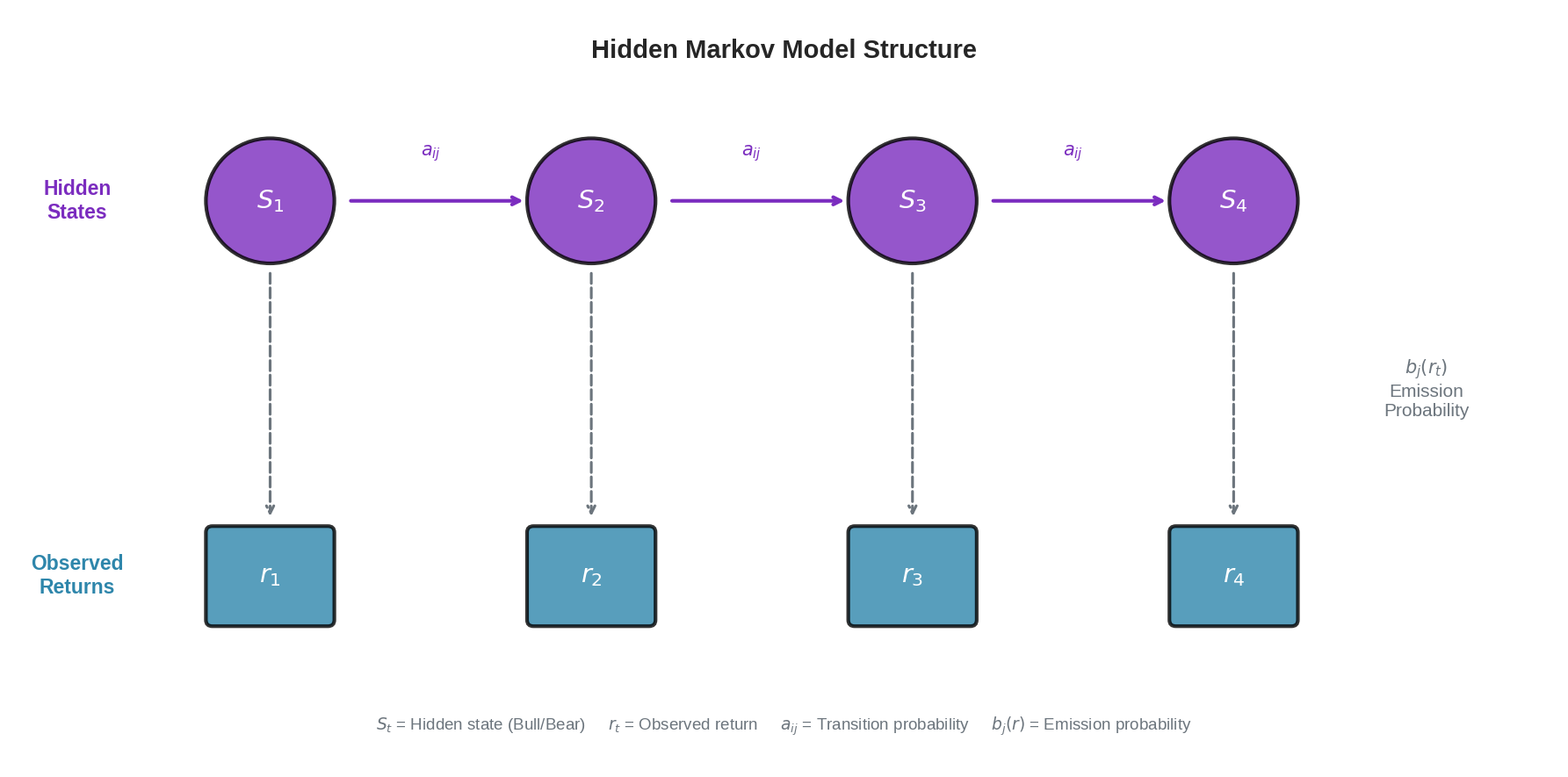
The diagram shows the core structure. At each time step:

• The market is in some hidden state S_t (Bull or Bear)

• We observe a return r_t generated by that state

• The state transitions to S_{t+1} according to transition probabilities a_ij

• The new state generates r_{t+1} according to emission probabilities b_j(r)

We never see the top row (states). We only see the bottom row (returns). The job of the HMM is to infer the hidden states from the observations.

---

Emission Distributions: How States Generate Returns

Each regime generates returns according to its own distribution. This is the emission distribution — given that we’re in state j, what’s the probability of observing return r?

For a two-state (Bull/Bear) model with Gaussian emissions:

Bull state:
  r ~ N(μ_bull, σ_bull²)
  Typical: μ = +0.05%/day, σ = 1.0%/day

Bear state:
  r ~ N(μ_bear, σ_bear²)
  Typical: μ = -0.10%/day, σ = 2.2%/day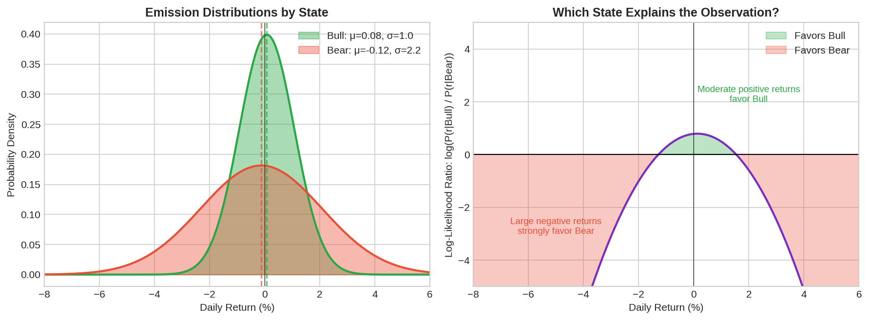

The left panel shows the two distributions. Bull (green) is centered slightly positive with low variance. Bear (red) is centered negative with high variance. There’s significant overlap — a return of -1% could plausibly come from either regime.

The right panel shows the log-likelihood ratio: log(P(r|Bull) / P(r|Bear)). Positive values mean the observation favors Bull; negative favors Bear.

A few key observations:

• Large negative returns (-4% or worse) strongly favor Bear

• Moderate positive returns (+1% to +2%) favor Bull

• Returns near zero are ambiguous

This is why single observations aren’t enough. A -1.5% day could be Bear, or it could be a bad day in a Bull market. We need to accumulate evidence over time.

---

Transition Probabilities: How States Evolve

The transition matrix A defines how the market moves between regimes:

         Bull(t+1)  Bear(t+1)
Bull(t)  [  0.98      0.02  ]
Bear(t)  [  0.05      0.95  ]

This says:

• If we’re in Bull today, 98% chance we stay Bull tomorrow, 2% chance we switch to Bear

• If we’re in Bear today, 95% chance we stay Bear, 5% chance we switch to Bull

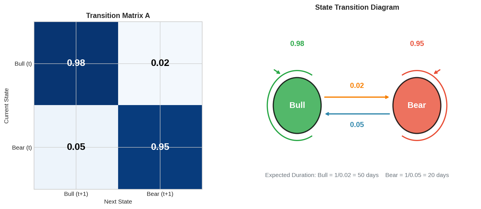
The left panel shows the matrix as a heatmap. The right panel shows the state diagram with transition arrows.

Expected state durations:

The expected time to stay in a state before switching is 1/(1-a_ii):

Bull duration: 1 / 0.02 = 50 days
Bear duration: 1 / 0.05 = 20 days

This matches the empirical observation that bull markets tend to be longer and slower, while bear markets are shorter and more violent.

Stationary distribution:

If the process runs long enough, what fraction of time is spent in each state? Solve πA = π:

π_bull × 0.98 + π_bear × 0.05 = π_bull
π_bull × 0.02 + π_bear × 0.95 = π_bear
π_bull + π_bear = 1

Solution: π_bull ≈ 0.71, π_bear ≈ 0.29

About 71% of the time in Bull, 29% in Bear. This is roughly consistent with historical market data.

---

The Forward Algorithm: Inference in Real Time

Given a sequence of observations, how do we compute the probability of being in each state? The forward algorithm does this efficiently.

Define the forward variable:

α_t(j) = P(r_1, r_2, ..., r_t, S_t = j)

This is the joint probability of seeing the observations up to time t AND being in state j at time t.

Initialization (t=1):

α_1(j) = π_j × b_j(r_1)

Where π_j is the initial state probability and b_j(r_1) is the emission probability of observing r_1 in state j.

Recursion (t > 1):

α_t(j) = b_j(r_t) × Σ_i [α_{t-1}(i) × a_ij]

In words: the probability of being in state j at time t equals:

• The probability of observing r_t in state j (emission)

• Times the sum over all previous states of: (being in that state) × (transitioning to j)

Posterior probability:

To get P(S_t = j | r_1, ..., r_t), normalize the forward variables:

P(S_t = j | observations) = α_t(j) / Σ_k α_t(k)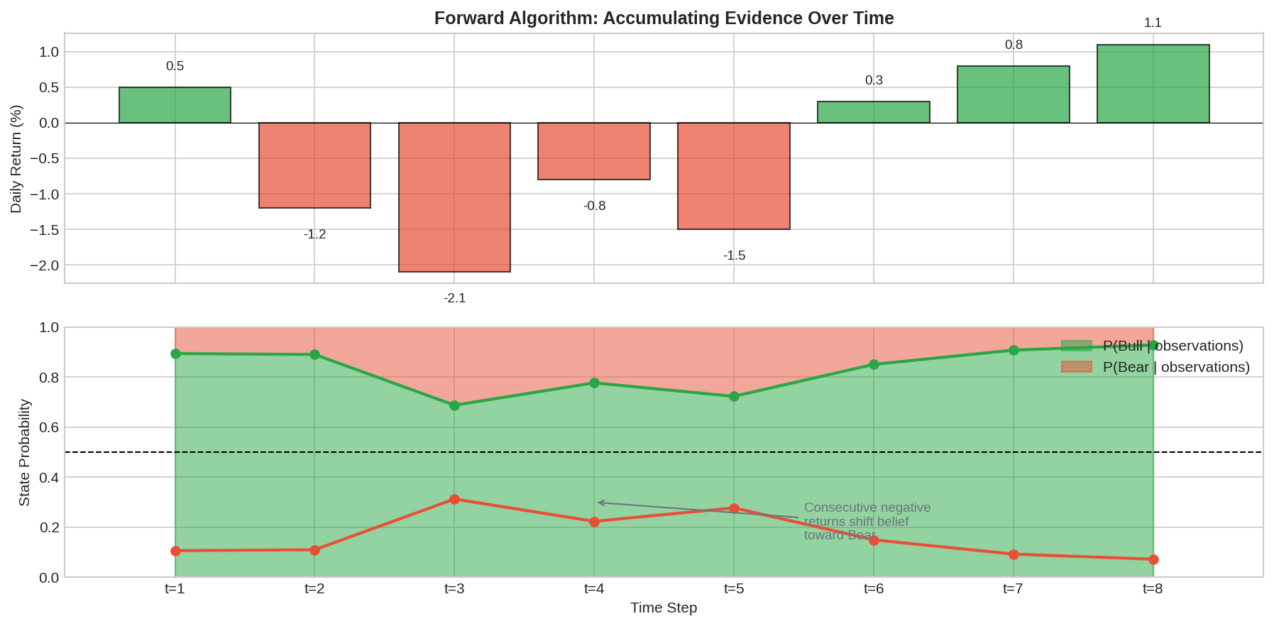

The chart shows the forward algorithm in action. The top panel shows a sequence of returns. The bottom panel shows how our belief about the current state evolves.

Starting from a prior belief of 80% Bull, the consecutive negative returns (t=2 through t=5) gradually shift the posterior toward Bear. By t=5, we’re about 70% confident in Bear. Then positive returns (t=7, t=8) shift us back toward Bull.

This is the key insight: the HMM accumulates evidence. No single observation flips the belief dramatically. It takes sustained evidence to overcome the prior and the transition probabilities.

---

The Complete Picture

Putting it all together with a longer simulation:

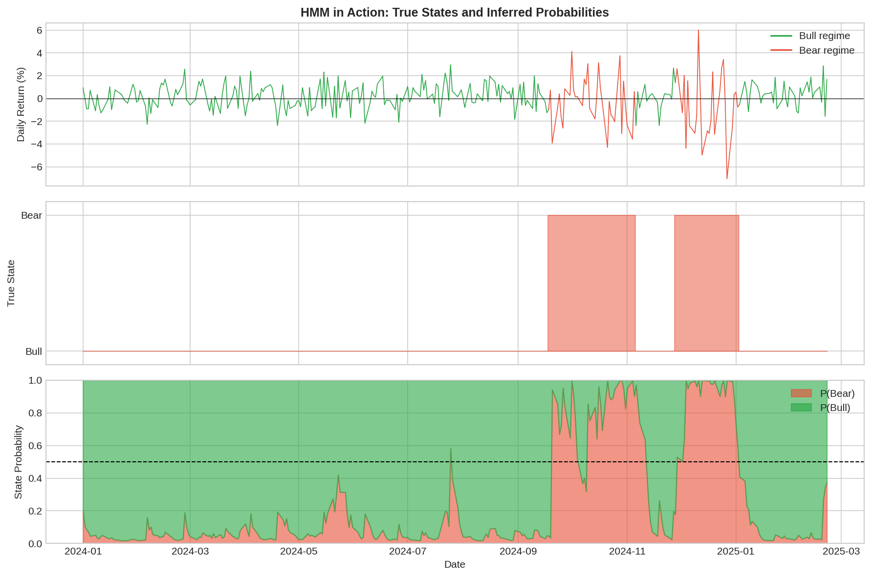
Top panel: Returns colored by true (hidden) state. Middle panel: The actual hidden state sequence. Bottom panel: Inferred state probabilities.

Notice several things:

1. The inference tracks the truth reasonably well. When the true state is Bear (middle panel shows 1), the inferred P(Bear) (red area in bottom panel) is generally high.

2. There’s lag at transitions. When the market switches from Bull to Bear, it takes several observations for the posterior to catch up. This is unavoidable—we need evidence to update beliefs.

3. There’s noise. Even within a regime, the posterior fluctuates. A single large negative return in Bull will temporarily increase P(Bear), even if we’re still in Bull.

4. The posterior rarely hits 0 or 1. We’re always somewhat uncertain. This is appropriate epistemic humility.

---

Parameter Estimation: The Baum-Welch Algorithm

So far, we’ve assumed we know the model parameters (transition matrix A, emission parameters μ and σ for each state). In practice, we estimate them from data.

The Baum-Welch algorithm (a special case of Expectation-Maximization) iteratively:

1. E-step: Given current parameters, compute the expected state occupancies and transitions using the forward-backward algorithm

2. M-step: Given expected states, update parameters to maximize likelihood

from hmmlearn.hmm import GaussianHMM

# Fit a 2-state HMM
model = GaussianHMM(n_components=2, covariance_type='full', n_iter=100)
model.fit(returns.values.reshape(-1, 1))

# Extract learned parameters
print("Transition matrix:")
print(model.transmat_)

print("Means:", model.means_.flatten())
print("Variances:", model.covars_.flatten())

Important: Baum-Welch finds a local maximum, not necessarily the global one. Results depend on initialization. In practice:

• Run multiple times with different random seeds

• Use domain knowledge to initialize (e.g., one state should have higher variance)

• Verify that learned parameters make economic sense

---

The Math: Formal Definition

For completeness, the formal HMM specification:

Model parameters λ = (A, B, π) where:

A = {a_ij}: Transition matrix
    a_ij = P(S_{t+1} = j | S_t = i)
    Constraints: a_ij ≥ 0, Σ_j a_ij = 1

B = {b_j(·)}: Emission distributions
    b_j(r) = P(r_t = r | S_t = j)
    For Gaussian: b_j(r) = N(r; μ_j, σ_j²)

π = {π_i}: Initial state distribution
    π_i = P(S_1 = i)
    Constraints: π_i ≥ 0, Σ_i π_i = 1

Three fundamental problems:

1. Evaluation: P(observations | λ)
   → Forward algorithm, O(T × N²)

2. Decoding: Most likely state sequence
   → Viterbi algorithm, O(T × N²)

3. Learning: Estimate λ from data
   → Baum-Welch algorithm, O(T × N² × iterations)

Where T = sequence length, N = number of states

---

Why HMMs Are the Default

HMMs became the standard for regime detection because:

1. Principled uncertainty quantification. Instead of “VIX > 25 = Bear,” we get P(Bear) = 0.73. This probability can inform position sizing, not just direction.

2. Automatic evidence accumulation. The forward recursion naturally weighs recent observations against prior beliefs and transition probabilities. No need to manually tune lookback windows.

3. Well-understood theory. The algorithms are efficient (O(T × N²)), the estimation procedure is standard, and the limitations are known.

4. Interpretable states. After fitting, you can inspect each state’s parameters and ask “does this look like a Bull market?” The states have economic meaning.

5. Generative model. You can simulate from the fitted HMM to do scenario analysis or stress testing.

---

The Chess Analogy

In chess, there’s a distinction between calculation and evaluation. Calculation is working out specific move sequences — if I play Nf3, they play Bb4, I play O-O, etc. Evaluation is assessing a position’s overall quality — who has better pieces, structure, king safety.

HMMs are evaluation tools, not calculation tools. They tell you “the current position is probably bullish” (evaluation), not “the market will drop 3% tomorrow” (calculation). This is a feature, not a bug. The market state is real and knowable in principle, even if future moves aren’t.

The question is: how quickly can we update our evaluation when the position changes? That’s the latency problem — Part 2.

---

Implementation

Full working code for fitting HMMs to market data:

import numpy as np
import pandas as pd
from hmmlearn.hmm import GaussianHMM

def fit_market_hmm(returns, n_states=2, n_iter=100):
    """
    Fit a Gaussian HMM to return series.
    
    Parameters:
        returns: pd.Series of daily returns
        n_states: number of hidden states (2 = Bull/Bear)
        n_iter: max EM iterations
    
    Returns:
        model: fitted HMM
        states: most likely state sequence
        probs: state probabilities at each time
    """
    # Reshape for hmmlearn
    X = returns.values.reshape(-1, 1)
    
    # Fit model
    model = GaussianHMM(
        n_components=n_states,
        covariance_type='full',
        n_iter=n_iter,
        random_state=42
    )
    model.fit(X)
    
    # Decode most likely states
    states = model.predict(X)
    
    # Get state probabilities
    probs = model.predict_proba(X)
    
    return model, states, probs


def interpret_states(model):
    """
    Identify which state is Bull vs Bear based on parameters.
    """
    means = model.means_.flatten()
    vols = np.sqrt(model.covars_.flatten())
    
    # Bear state typically has higher volatility
    bear_state = np.argmax(vols)
    bull_state = 1 - bear_state
    
    print(f"Bull state (#{bull_state}):")
    print(f"  Mean: {means[bull_state]:.4f}")
    print(f"  Volatility: {vols[bull_state]:.4f}")
    print(f"\nBear state (#{bear_state}):")
    print(f"  Mean: {means[bear_state]:.4f}")
    print(f"  Volatility: {vols[bear_state]:.4f}")
    
    print(f"\nTransition matrix:")
    print(f"  P(Bull→Bull): {model.transmat_[bull_state, bull_state]:.3f}")
    print(f"  P(Bull→Bear): {model.transmat_[bull_state, bear_state]:.3f}")
    print(f"  P(Bear→Bull): {model.transmat_[bear_state, bull_state]:.3f}")
    print(f"  P(Bear→Bear): {model.transmat_[bear_state, bear_state]:.3f}")
    
    return bull_state, bear_state


# Example usage
if __name__ == "__main__":
    # Generate synthetic data
    np.random.seed(42)
    n = 500
    
    # True states
    states = np.zeros(n, dtype=int)
    for t in range(1, n):
        if states[t-1] == 0:
            states[t] = np.random.choice([0, 1], p=[0.98, 0.02])
        else:
            states[t] = np.random.choice([0, 1], p=[0.05, 0.95])
    
    # Generate returns
    returns = np.where(states == 0,
                       np.random.randn(n) * 1.0 + 0.05,
                       np.random.randn(n) * 2.2 - 0.10)
    returns = pd.Series(returns)
    
    # Fit HMM
    model, pred_states, probs = fit_market_hmm(returns)
    
    # Interpret
    bull_idx, bear_idx = interpret_states(model)
    
    # Accuracy
    accuracy = np.mean(pred_states == states)
    print(f"\nState prediction accuracy: {accuracy:.1%}")

All code is open source — use it, modify it, build on it. No guarantees about correctness or performance. Test everything yourself before deploying with real capital.

---

Summary

Hidden Markov Model
  Framework for inferring unobservable states from observations.
  States evolve via transition matrix, generate observations via emissions.

Emission distributions
  Each state has its own return distribution.
  Bull: positive mean, low vol. Bear: negative mean, high vol.

Transition matrix
  Encodes persistence. States are sticky (a_ii ≈ 0.95-0.98).
  Expected duration = 1/(1-a_ii).

Forward algorithm
  Computes P(state | observations seen so far) in O(T × N²).
  Accumulates evidence over time.

Baum-Welch
  EM algorithm for parameter estimation.
  Finds local maximum; run multiple times.

Why HMMs
  Principled uncertainty, evidence accumulation, interpretable.
  The default tool for regime detection.

---

Coming up:

• Part 2: The Latency Problem — How long does it take to detect a regime change? The unavoidable detection lag.

• Part 3: Beyond HMMs — Changepoint detection, machine learning, and what I’m actually implementing.

---

HMMs are powerful but not magic. They can’t predict regime changes before they start — only detect them after evidence accumulates. Understanding this limitation is critical for setting realistic expectations. More on this in Part 2.

But remember: Alpha is never guaranteed. And the backtest is a liar until proven otherwise.

The material presented in Math & Markets is for informational purposes only. It does not constitute investment or financial advice.

---