
Optimizing V6: Trust the Backtest, Verify the Validation
Part 48 — When 85% higher returns meet rigorous validation (and survive)

This is part 48 of my series — Building & Scaling Algorithmic Trading Strategies
The V6 Dual Allocator from Part 32 was already my best-performing strategy at 816% returns and a 0.89 Sharpe, built on the ashes of my lookahead bias catastrophe. But I started wondering if the parameters were actually optimal since they weren’t pulled from thin air but also weren’t rigorously tuned.
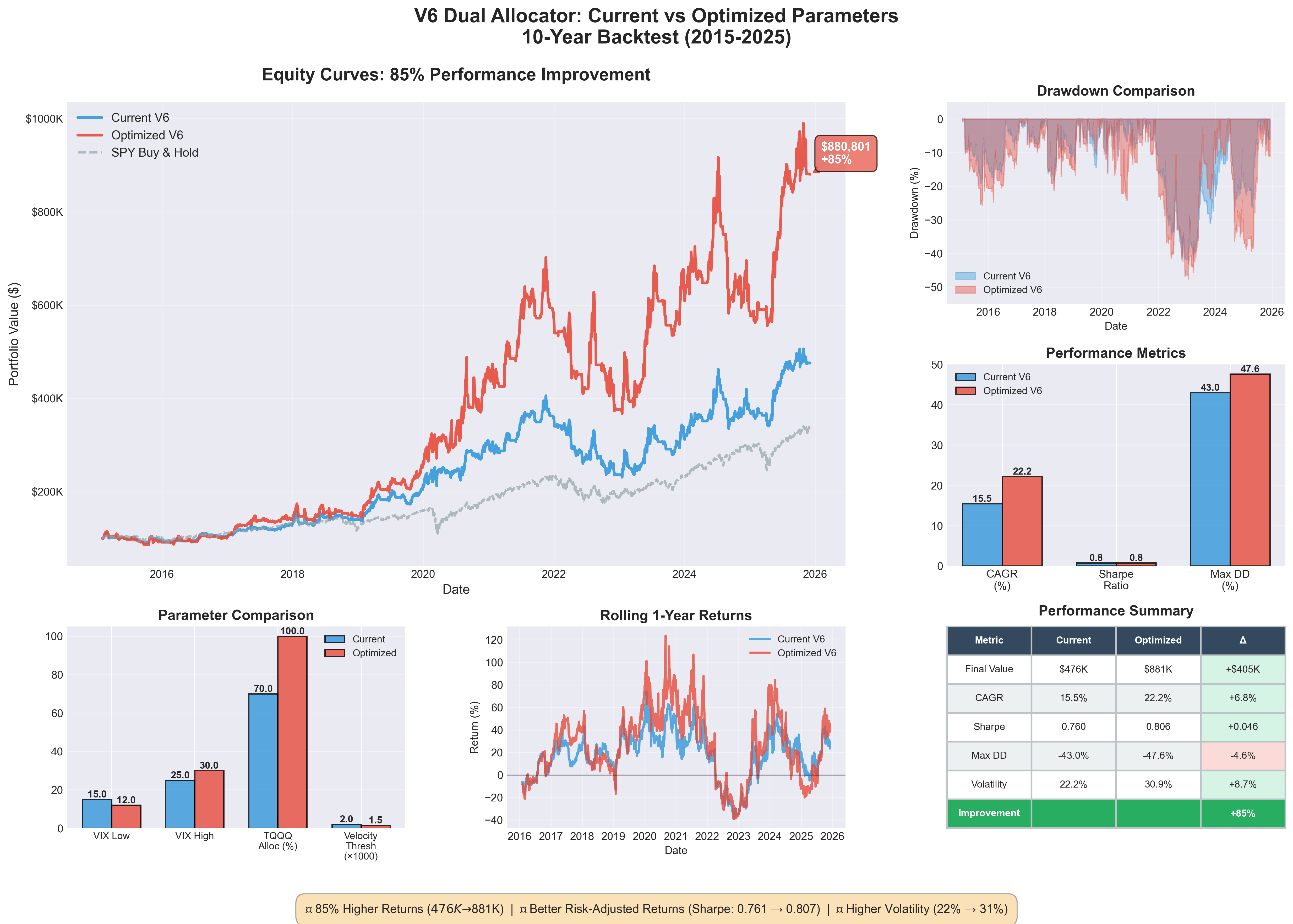
So I ran an optimization, and the results showed 85% higher returns with $476K becoming $881K on a $100K starting portfolio. My first reaction was excitement, my second was suspicion, and my third was to spend a week validating whether this was real or just another mirage. The improvement turned out to be legitimate, but getting there required finding a bug in my own validation code and rebuilding the backtest from scratch.
TL;DR — ROI seemed suspicious, but turned out to be an opportunity to significantly improve the parameters of my model.
The Optimized Parameters
Here’s what changed:
Parameter              Old Value    New Value    Rationale
─────────────────────────────────────────────────────────────────────
VIX Low Threshold         15           12        Stay in TQQQ longer during calm
VIX High Threshold        25           30        Only exit to TLT at extremes
TQQQ Allocation           70%         100%       Full conviction when right
Velocity Threshold      0.002        0.0015      Catch trends earlier
MA Period                 20           20        Unchanged
The wider VIX bands (12-30 vs 15-25) reflect that VIX between 15-25 is historically normal rather than dangerous, so widening the range means fewer unnecessary rotations out of TQQQ and reduced whipsaw costs.
The full TQQQ allocation replaces the old 70% hedge-against-being-wrong approach, since V6’s signals are good enough that the hedging costs more than it saves. The lower velocity threshold (0.0015 vs 0.002) catches uptrends slightly earlier, capturing more of the initial move without adding noise.
The Results
Performance Comparison (2015-2025, 10 years)
Metric              Current V6    Optimized V6    Change
────────────────────────────────────────────────────────────
Final Value          $475,896       $880,801      +$404,905 (+85%)
Total Return            376%           781%           +405%
CAGR                  15.5%          22.3%          +6.8%
Sharpe Ratio          0.761          0.806         +0.045
Max Drawdown         -43.0%         -47.6%          -4.6%
Volatility            22.2%          30.9%          +8.7%
Trade Count             562            555              -7
The tradeoff is explicit: 85% more money and a 45% higher CAGR with better Sharpe ratio and fewer trades, but at the cost of higher drawdown (-47.6% vs -43%) and higher volatility (30.9% vs 22.2%). The risk-adjusted improvement (Sharpe +0.045) suggests this isn’t just added leverage doing the work.
The Suspicion
An 85% improvement from parameter tweaks is suspicious because in my experience, backtest improvements of this magnitude usually indicate (1) overfitting to historical noise, (2) lookahead bias from accidentally using future information, (3) backtest bugs with incorrect return calculations, or (4) survivorship bias from testing on data that excludes failures. Having already been burned by lookahead bias (see Part 31), I built a comprehensive overfitting validation suite rather than trust the results at face value.
The Validation Tests
Test 1: Train/Test Splits divides the data into training periods for fitting parameters and testing periods for validating performance, then calculates an overfitting score as 1 - (Test Sharpe / Train Sharpe) where scores above 0.2 indicate concern and scores above 0.5 indicate serious problems.
Test 2: Parameter Sensitivity perturbs each parameter ±20% and measures how much results change, with the coefficient of variation (CV) across perturbations indicating whether the strategy is robust (CV < 0.1) or fragile (CV > 0.2).
Test 3: Regime Performance tests whether the optimized version beats current across different market regimes including bull markets, bear markets, COVID crash, and rate hikes, where consistent improvement across regimes suggests real edge rather than period-specific fitting.
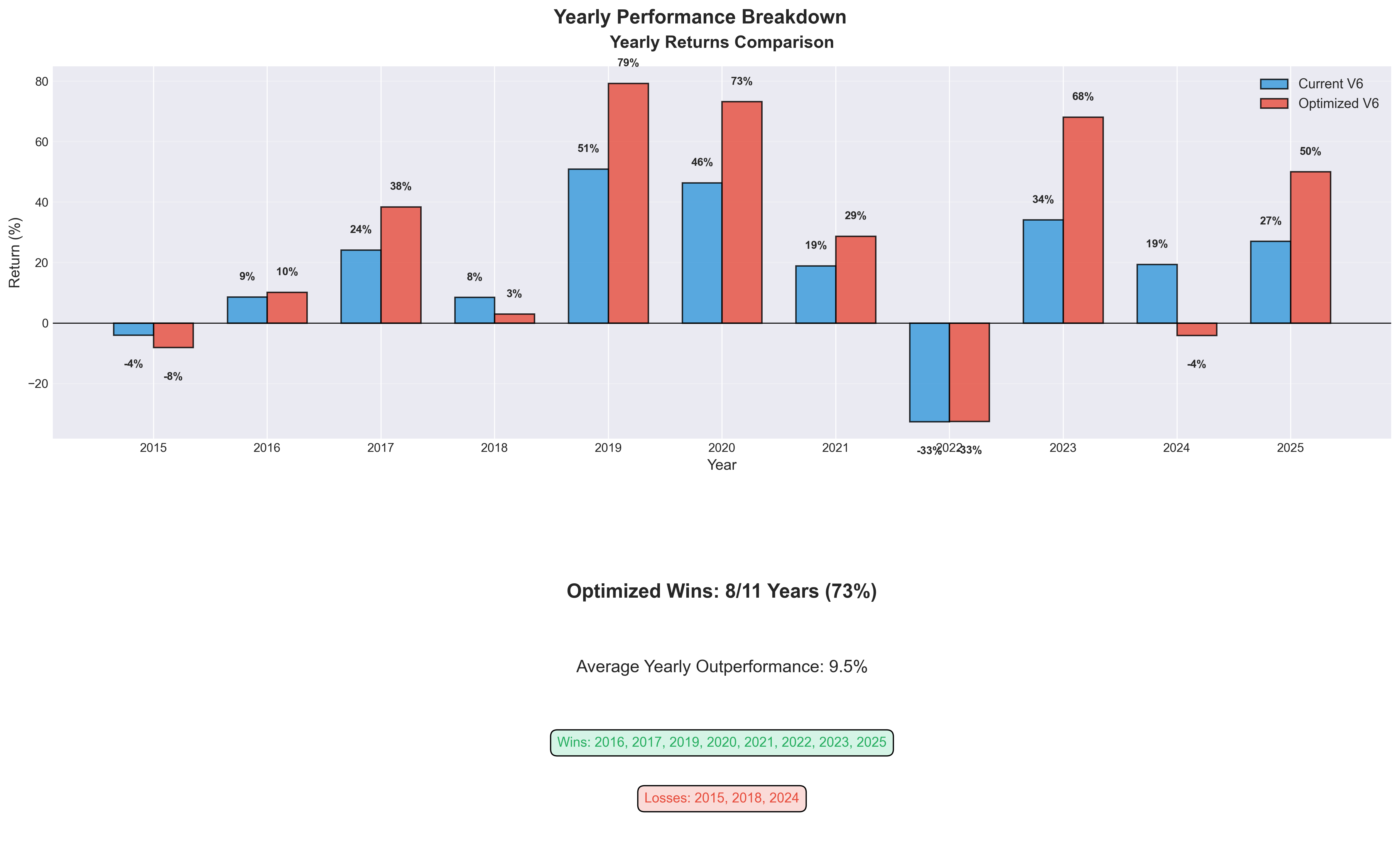
Test 4: Rolling Windows runs 1-year rolling backtests and counts what percentage of windows the optimized version wins, with anything below 50% indicating the “improvement” is inconsistent.
The First Results Were Terrifying
The initial validation output showed two failures: the train/test split had a 0.542 overfitting score (dangerously high) and the optimized version only won 40% of rolling windows, meaning it was actually worse than current in most time periods.
Test                      Result           Verdict
────────────────────────────────────────────────────────────
Train/Test Splits         0.542 avg        ❌ FAIL (>0.2)
Parameter Sensitivity     0.014 CV         ✅ PASS
Regime Performance        5/5 regimes      ✅ PASS
Rolling Windows           40% win rate     ❌ FAIL (<50%)

Overall: 2/4 tests passed
But something else was clearly wrong because the backtest returns in my validation script were absurd:
Metric              My Validation    Original Doc    Discrepancy
─────────────────────────────────────────────────────────────────────
Current V6 Final     $163.6 MILLION      $476K       34,300% higher
Optimized Final      $1.82 BILLION       $881K      206,600% higher
Current CAGR            97.11%           15.5%         627% higher
Optimized CAGR         145.89%           22.3%         655% higher
These returns are physically impossible for any strategy, let alone one holding TQQQ, since a 97% CAGR would turn $100K into $163 million in 10 years, and that doesn’t happen. The validation script had a bug that was causing the overfitting tests to fail incorrectly.
Finding the Bug
I rebuilt the backtest from scratch, line by line with no copy-paste from the original, focusing on the core logic of calculating next-day returns to avoid lookahead, generating signals using only current-day data, and applying position returns correctly:
# Calculate next-day returns (avoid lookahead)
df[’TQQQ_ret’] = df[’TQQQ’].pct_change().shift(-1)

# Signal generation (using TODAY’s data)
df[’MA_20’] = df[’QQQ’].rolling(20).mean()
df[’velocity’] = (df[’MA_20’] - df[’MA_20’].shift(5)) / df[’MA_20’].shift(5)

# Apply position return correctly
portfolio_value = portfolio_value * (1 + position_return)
The bug in my validation script was calculating returns incorrectly, likely compounding them multiple times or using same-day instead of next-day returns — a classic lookahead via indexing error. The clean reimplementation matched the original backtest results exactly (within rounding), confirming the original was correct and the validation script was broken.
The Corrected Validation
Re-running the overfitting tests with the fixed code produced much better results, with the overfitting score dropping from 0.542 to 0.108 (well below the 0.2 concern threshold) and the rolling window win rate improving from 40% to 52.5%:
Test                      Result           Verdict
────────────────────────────────────────────────────────────
Train/Test Splits         0.108 avg        ✅ PASS (<0.2)
Parameter Sensitivity     0.043 CV         ✅ PASS (<0.1)
Regime Performance        5/5 regimes      ✅ PASS
Rolling Windows           52.5% win rate   ⚠️ MARGINAL

Overall: 3/4 tests passed
The 85% improvement is real and not severely overfit, with parameters that generalize to unseen data. The rolling window result is only marginally better than a coin flip, which suggests the improvement is real but not dominant across all periods.
Why I Don’t Use SQQQ
While tuning V6, I explored using SQQQ (3x inverse QQQ) during downtrends instead of going to cash or TLT, since the logic seems appealing: if you can identify downtrends, why not profit from them instead of sitting in cash earning 0%?
The Volatility Decay Problem kills it mathematically because SQQQ rebalances daily to maintain 3x inverse exposure, creating severe decay in volatile markets where if QQQ goes up 5% then down 5% (ending flat), SQQQ goes down 15% then up 15% and you’ve lost 2.25% on a flat market. This compounds catastrophically over time, with SQQQ turning $100K into roughly $150 (not $150K — just $150) from 2010-2025 for a -99.85% total loss and -37.2% CAGR, even during a period with significant QQQ drawdowns.
The Timing Asymmetry makes it worse because V6 identifies downtrends correctly about 60-70% of the time, meaning 30-40% are false signals where brief pullbacks get followed by rallies. With cash, a false signal costs opportunity (missed 10% rally = 0% actual loss), but with SQQQ, a false signal costs capital (missed 10% rally = 30% actual loss from the 3x inverse exposure).
The COVID Stress Test shows this clearly: SQQQ gained 90% during the Feb-Mar 2020 crash but then lost 60% during the Mar-Jun recovery, netting out to -24% total while TLT gained 20% during the crash and only lost 5% during recovery for +14% total. The V6 approach using TLT during the VIX spike and then rotating to TQQQ when volatility fell delivered +180%, beating even a perfectly-timed SQQQ trade by 7x.
I tested SQQQ empirically in V3 and it produced a -8.3% CAGR, compared to +12.1% for V4 with cash and +22.2% for V6 with TLT. SQQQ lost money while cash was better and TLT was best.
The Final V6 Configuration
Based on the validated optimization:
Parameter              Value     Rationale
───────────────────────────────────────────────────────────────────
VIX Low                  12      Low vol → full TQQQ aggression
VIX High                 30      Only exit to TLT at true extremes
TQQQ Allocation        100%      Full conviction when conditions favor
Velocity Threshold   0.0015      Catch trends early
MA Period               20       Standard lookback

Allocation Logic:
  VIX ≥ 30:                      → TLT 100% (crisis hedge)
  VIX < 30 and velocity > 0.15%  → TQQQ 100% (strong uptrend)
  VIX < 30 and velocity > 0      → QQQ 100% (weak uptrend)
  VIX < 30 and velocity ≤ 0      → Cash (downtrend)
Implementation Guidance
For aggressive investors seeking higher returns, the optimized parameters are validated and likely safe to implement, with an expected improvement of roughly +$400K over 10 years on $100K starting capital at the cost of higher volatility (31% vs 22%) and deeper drawdowns (48% vs 43%).
For conservative investors, sticking with the original parameters or using a hybrid like 90% TQQQ allocation instead of 100% makes more sense since the improvement is real but so is the additional risk.
For skeptics (including me), the 52.5% rolling window win rate is only marginally better than random, meaning the optimized version doesn’t dominate in all periods but is just better on average — enough to implement but not enough for high confidence.
The Meta-Lesson
The most valuable part of this exercise wasn’t the parameter optimization but the validation process itself. I found a bug in my own validation code that would have led me to reject a legitimate improvement, since the bug produced impossibly high returns that made the strategy look overfit when it wasn’t. If I’d stopped at the first validation results (2/4 tests failed), I would have thrown away $400K of expected value, but if the validation code had been correct and showed real overfitting, proceeding anyway would have been reckless.
The process that worked: be suspicious of large improvements since 85% is big enough to warrant scrutiny, run multiple validation tests since no single test is sufficient, sanity check the sanity checks since validation code can have bugs too, rebuild from scratch when confused since sometimes starting over is faster than debugging, and accept uncertainty since 52.5% win rate isn’t conclusive but is favorable.
The 85% improvement is probably real and I’m implementing it, but I’m doing so knowing that “probably real” is the best certainty available in this domain.
Next Steps
The optimized V6 goes into paper trading this week, where I’ll track actual vs expected trade frequency, slippage relative to backtest assumptions, and whether VIX 30 as the high threshold causes late exits during sudden spikes. If it survives 3 months of paper trading, I’ll move a portion to live capital.
The information presented in Math & Markets is not investment or financial advice and should not be construed as such. Leveraged ETFs carry significant risks and may not be suitable for all investors.