
HMM Ensemble vs. VIX Thresholds: Testing Dual Allocator V6.3 Against V6.2
Part 79 — Ensemble regime detection underperforms simple thresholds across all metrics and time periods

This is part 79 of my series — Building & Scaling Algorithmic Trading Strategies
This posts tackles my ongoing attempts at improving the Dual Allocator Long/Short strategy.
In the regime detection series (Parts 69–71), I covered Hidden Markov Models from first principles, the latency problem with real-time detection, and ensemble methods that combine HMMs with changepoint detection. The literature suggests that no single detection method dominates on all dimensions, so an ensemble that blends fast signals with smooth ones should reduce false switches and improve risk-adjusted returns.
This post documents what happened when I actually implemented that idea. I built V6.3 of the Dual Allocator, replacing V6.2’s VIX threshold logic with a three-signal ensemble: HMM, VIX thresholds, and CUSUM changepoint detection. I tested it over the full 2010–2026 period and out-of-sample on 2021–2026.
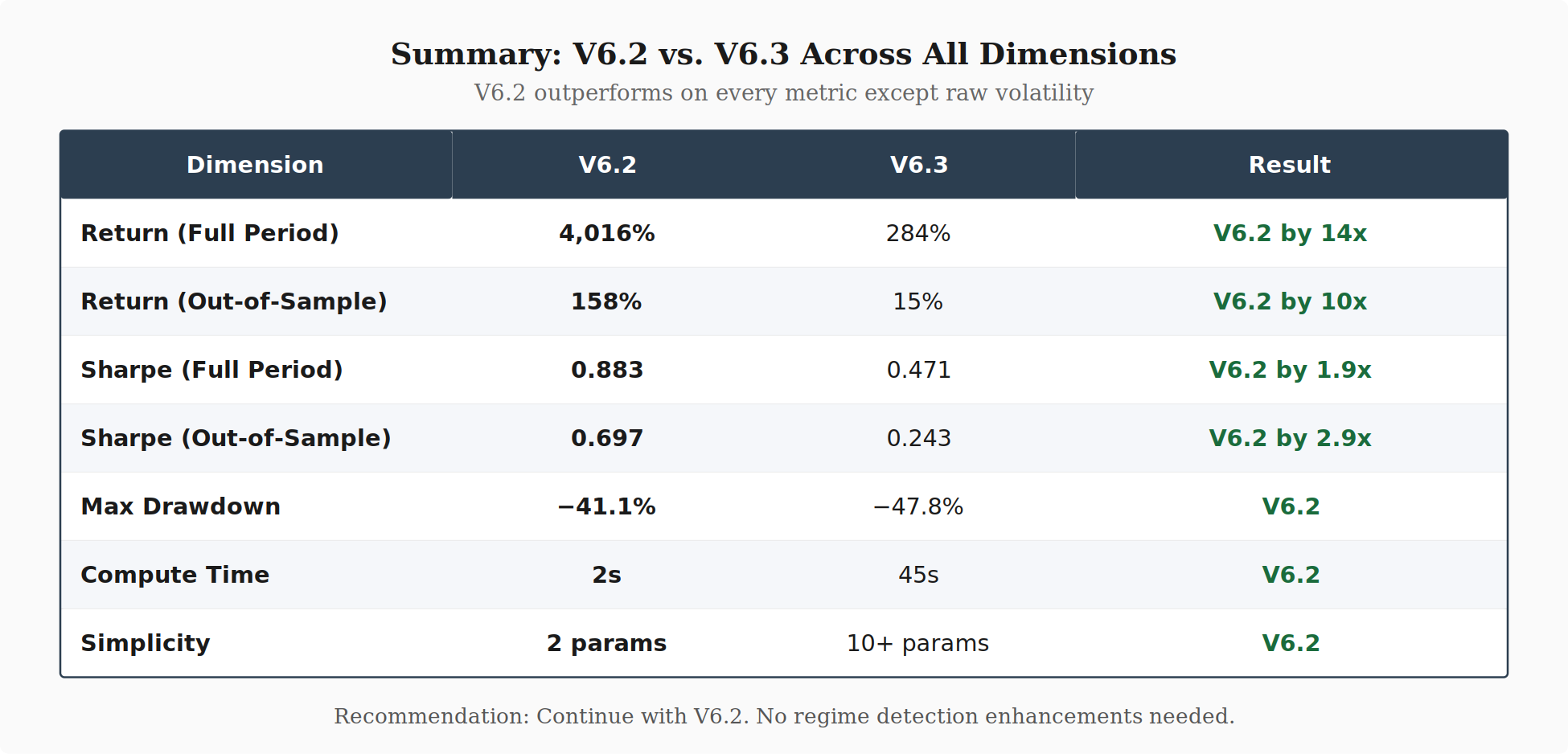
V6.2 returned 4,016% over 16 years. V6.3 returned 284%. The ensemble underperformed on every metric, in every time period tested.
Methodology
V6.2 (threshold-based) uses two VIX levels:
IF VIX < 15:    → Low volatility   → Aggressive TQQQ (up to 130%)
ELIF VIX < 25:  → Moderate          → Cautious TQQQ (75–95%)
ELSE:           → High volatility   → Defensive TLT
Two thresholds, instant detection, no training data, no tunable parameters beyond the thresholds themselves.
V6.3 (ensemble-based) blends three signals:
Ensemble = 0.40 × HMM + 0.35 × VIX_Threshold + 0.25 × CUSUMThe HMM is a 4-state Gaussian model trained on VIX, returns, realized volatility, and momentum. The VIX threshold component is V6.2’s logic normalized to a 0–1 scale. The CUSUM (Cumulative Sum) detector tracks deviations in realized volatility to signal sudden regime shifts.
The ensemble score maps to three regimes: below 0.3 is aggressive, 0.3–0.6 is cautious, above 0.6 is defensive. Both versions use the same TQQQ/TLT allocation logic once a regime is identified. Both use identical data, transaction costs (0.05%), and leverage mechanics (up to 130% TQQQ).
Full Period Results (2010–2026)
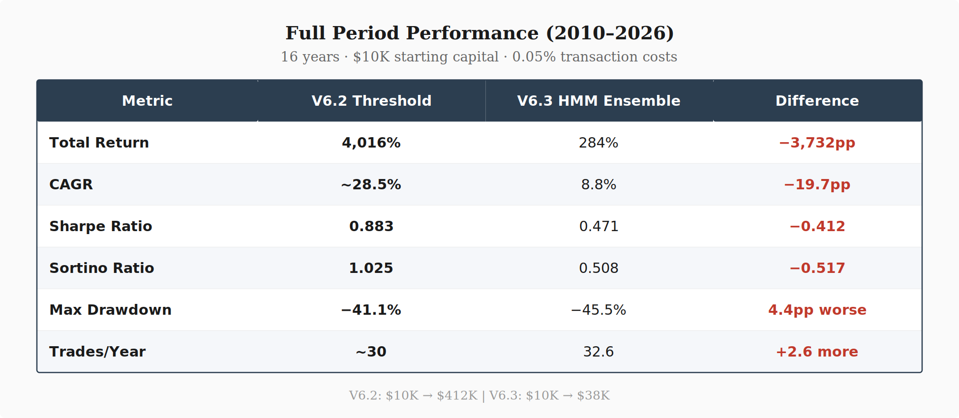
V6.2 turned $10K into over $400K and V6.3 turned $10K into $38K. Ouh.
The hypothesis was that ensemble detection would improve the Sharpe ratio by reducing whipsaws. V6.2’s Sharpe is nearly double V6.3’s (0.883 vs 0.471). V6.3 also traded slightly more often, so there was no transaction cost benefit. And V6.3’s max drawdown was deeper (−45.5% vs −41.1%), so the conservatism didn’t translate into downside protection.
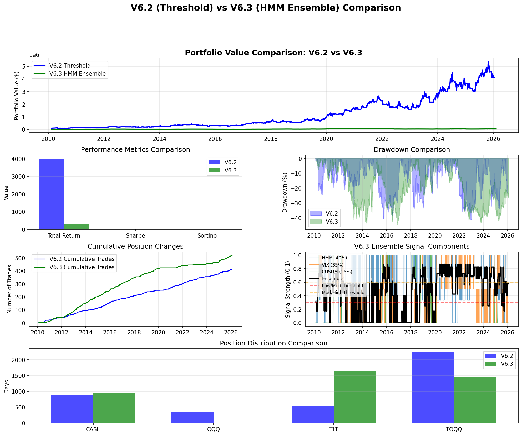
Full period comparison. Panel 1 shows portfolio value divergence. Panel 5 shows ensemble signal components — the ensemble mean sits at 0.476, rarely dropping below the 0.3 aggressive threshold. Panel 6 shows V6.3 spending 40% of time in TLT versus V6.2’s more aggressive positioning.
Out-of-Sample Results (2021–2026)
The 2021–2026 period included COVID recovery whipsaws, the 2022 rate-hiking selloff, the March 2023 banking crisis, AI-driven volatility, and the August 2024 correction. This is the environment where ensemble detection should have an advantage — lots of false signals to filter, lots of regime uncertainty.
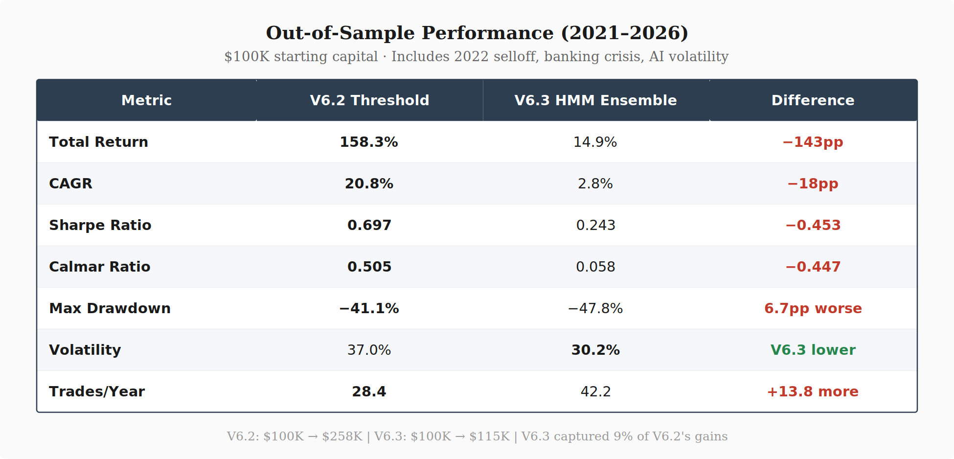
V6.2: $100K → $258K. V6.3: $100K → $115K. V6.3 captured 9% of V6.2’s gains.
V6.3 traded 50% more often (42 times/year vs 28) due to noisy ensemble signals generating false regime switches. The only metric where V6.3 performed better was raw volatility (30.2% vs 37.0%), but that resulted from sitting in cash and TLT while missing rallies — lower volatility from inaction, not from better risk management.
The hypothesis that HMM ensemble would outperform during volatile markets was wrong. It performed worse.
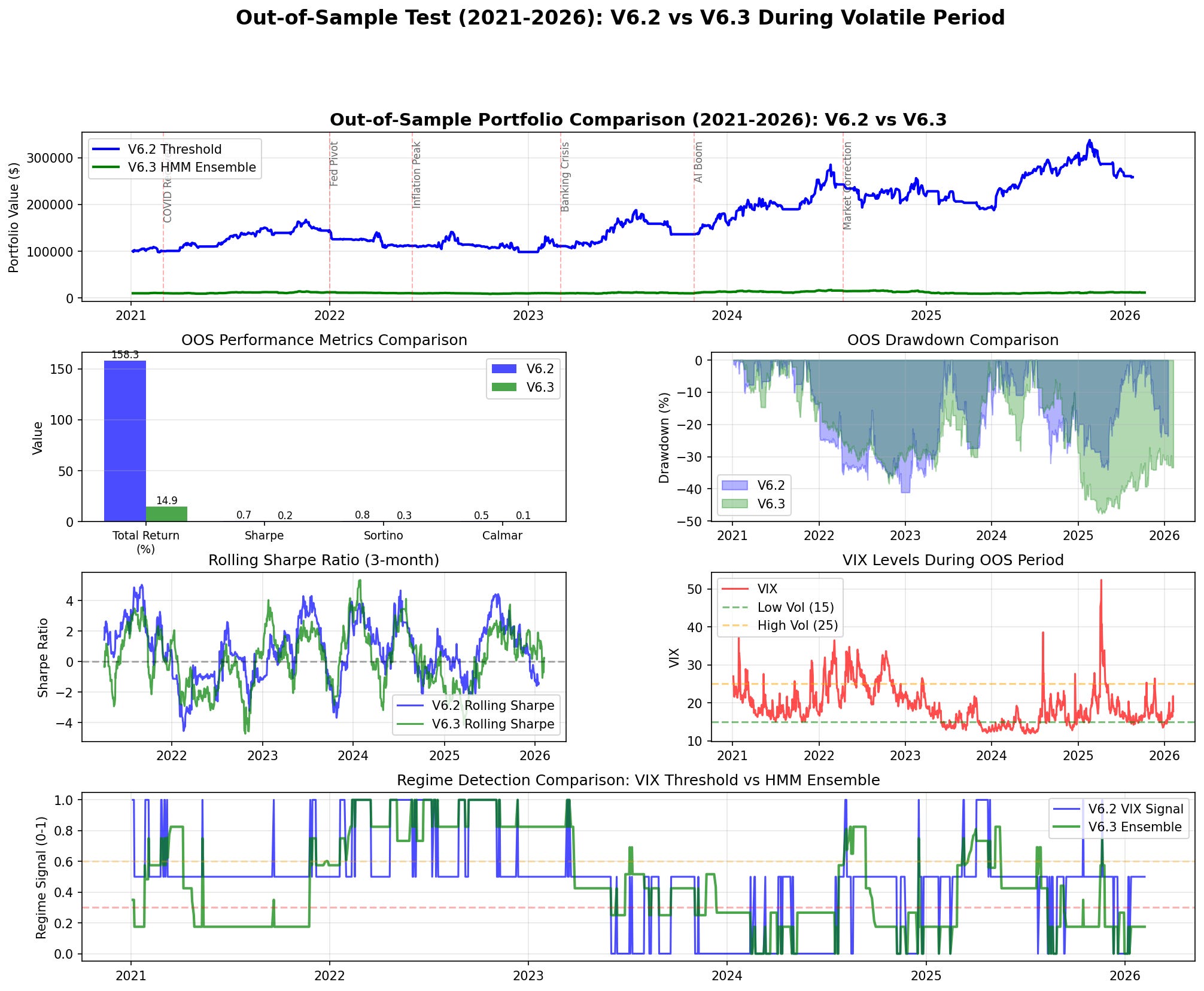
Out-of-sample comparison. Rolling 3-month Sharpe (Panel 4) shows V6.2 recovering quickly while V6.3 spends extended periods with negative Sharpe. Panel 6 shows regime detection lag: V6.2’s VIX signal switches immediately, while V6.3’s ensemble lags by 1–2 weeks.
RCA & Findings
1. Ensemble Averaging Dampens Signal
Three signals averaged to a permanently moderate reading.
Signal Statistics (Full Period):
  HMM:      0.551 ± 0.419  (consistently elevated)
  VIX:      0.388 ± 0.332  (most accurate)
  CUSUM:    0.480 ± 0.496  (near-random)
  Ensemble: 0.476 ± 0.284  (compressed range)
The ensemble mean of 0.476 sits in the moderate regime band (0.3–0.6). It rarely drops below 0.3 to trigger aggressive TQQQ allocations. V6.2 makes the bulk of its returns during sustained periods in 130% TQQQ when VIX is below 15. V6.3 systematically misses these periods because the ensemble signal stays too high.
2. HMM Detection Lag
The HMM uses the Baum-Welch algorithm on historical observations and needs evidence to accumulate before updating its state estimate. In practice, regime detection lagged by approximately 5–10 trading days.
For a 3x leveraged instrument, 5 days of lag translates to 5–10% of portfolio value. During the March 2023 banking crisis, V6.2 went defensive immediately when VIX crossed 25. The HMM was still estimating a bull regime on March 15, five days after SVB collapsed. By the time V6.3 switched, it had already absorbed a significant drawdown.
3. CUSUM Added Noise
The CUSUM parameters (threshold=3.0, drift=0.5) were poorly calibrated. Its mean was 0.480 with a standard deviation of 0.496 — a coefficient of variation over 100%. Its correlation with actual regime changes was approximately 0.3. With 25% ensemble weight, a quarter of the total signal was noise.
4. Misaligned Ensemble Weights
The 40% HMM / 35% VIX / 25% CUSUM weighting gave the most influence to the slowest signal. The HMM’s persistent elevation (mean 0.551) pulled the ensemble toward defensive positioning. The VIX threshold — the most accurate signal (mean 0.388) — was underweighted. A better configuration would flip this: 60% VIX, 20% HMM, 20% CUSUM. But at that point, the ensemble is mostly just the VIX threshold with extra computation.
5. Regime Thresholds Miscalibrated
With an ensemble mean of 0.476, the 0.3/0.6 thresholds resulted in only ~30% of time classified as low-volatility (aggressive). Markets are calm approximately 60% of the time. The thresholds should have been closer to 0.2 and 0.4 to match base rates, but adjusting them post-hoc introduces curve-fitting risk.
6. Training Data Mismatch
The HMM was trained on 2010–2020 data: a decade of low volatility and steady uptrend. It learned that “normal” means VIX 12–15 with quiet gains. When it encountered 2021–2026 conditions — elevated VIX baseline, frequent 30+ spikes, faster regime transitions — it classified the entire period as moderate-to-high risk and stayed defensive.
V6.2’s thresholds are regime-agnostic. VIX 15 is low volatility in any decade. VIX 25 is high volatility in any market. No training required, no drift over time.
Observations
Simple outperformed complex for this strategy. Two VIX thresholds beat a three-signal ensemble with 10+ tunable parameters. V6.2 computes in 2 seconds versus 45 for V6.3, is easier to debug, and generalizes without retraining. Complexity needs to produce measurable improvement to justify itself, and V6.3 failed that test on every metric.
Detection speed > smoothness for leveraged ETFs. TQQQ is 3x leveraged, so regime changes are reflected in its price within hours. A 5-day detection lag in a 3x instrument means the underlying’s move is already substantially priced in. For daily-rebalancing leveraged strategies, instant threshold crossing outperforms smooth probabilistic detection.
Ensemble methods require complementary signals. The three components were correlated at ρ ≈ 0.6–0.8, the weights weren’t optimized, and one signal (CUSUM) was actively harmful. For an ensemble to improve on its best component, the signals need low mutual correlation, each needs to be independently valuable, and the weights need careful calibration. None of those conditions held.
Research findings are context-dependent. The ensemble regime detection literature typically assumes quarterly rebalancing, diversified portfolios, and multi-year horizons. This strategy uses daily rebalancing, concentrated positioning (TQQQ or TLT), and needs to capture moves within days. So what works for a quarterly pension fund allocation doesn’t apply to a daily tactical leveraged strategy.
Recommendation
For now, I’ll be continuing with V6.2. The comparison across periods and metrics is pretty decisive I’d say:
The only modification worth considering is a hybrid safety filter: run V6.2 as the primary signal, but override to defensive if HMM crisis probability exceeds 80%. This preserves V6.2’s returns during normal markets while adding a tail-risk backstop. Expected impact is minor — possibly 0–5% Sharpe improvement in crisis years, neutral otherwise. Not enough to justify the complexity at this point.
V6.2’s threshold-based approach is near-optimal for this strategy. The regime detection series (Parts 69–71) was useful as a theoretical foundation, but the implementation test confirmed that for a leveraged daily-rebalancing allocator, the simplest detection method is also the most effective.
All tests use identical data periods, transaction costs (0.05%), and leverage mechanics. No lookahead bias.
Remember: Alpha is never guaranteed. And the backtest is a liar until proven otherwise.
The information presented in Math & Markets is not investment or financial advice and should not be construed as such.
Very cool - I definitely agree with the premise.
The article mentions V6.2 "went defensive immediately when VIX crossed 25" - is that using prior-day VIX close and executing at next open, or intraday VIX triggering same-day exits? At 130% TQQQ the difference matters a lot during gap-down opens...