
Half-Lives of Alpha: Why Every Strategy Eventually Dies
Part 80 — Decay Series 1 of 3 —The mathematics of signal decay, and my experience on the shelf life of edge

This is part 80 of my series — Building & Scaling Algorithmic Trading Strategies
The Problem I Keep Running Into
Over the past 79 posts, I’ve built, tested, and killed more strategies than I care to count. A VIX term structure arbitrage that looked beautiful until I fixed the lookahead bias. An ML model that “learned” to exploit a data bug and produced imaginary 6,000% returns. A Recession Anxiety Index that turned out to be buy-and-hold with extra steps.
Every one of these followed the same arc: discover a signal, get excited about the backtest, dig deeper, discover it doesn’t work — or works far less well than it appeared.
I used to think this was my problem. Bad code, sloppy methodology, insufficient rigor. And some of it was (hello, lookahead bias). But the pattern is too consistent and too universal to be purely personal. There’s a deeper dynamic at work.
Strategies decay — all of them. The question isn’t whether your edge will erode — it’s how fast and why. And unless you have a framework for thinking about this, you’re flying blind.
This is Part 1 of a 3-part series on the mathematics of strategy decay:
Part 1 (this post): Half-lives of alpha — the empirical evidence and mathematical framework
Part 2: Monitoring a live strategy — statistical tests for detecting structural breaks
Part 3: Adaptive strategies — can a strategy evolve, or is that just overfitting in real-time?
My Own Strategy Graveyard
Before we get to the theory, let me show you the data I’ve accumulated involuntarily.
Here’s what happened across six versions of my dual allocator strategy:
V1 through V4: the backtest always looked better than reality. V5: the ML model found the bug, not the signal. V6: the first version where backtest and reality converge.
The pattern across V1–V5 is textbook:
Version    What Happened                              Backtest   Reality    Gap
─────────────────────────────────────────────────────────────────────────────────
V1         Initial momentum strategy                     35%       12%     -66%
V2         "Optimized" parameters                        55%       18%     -67%
V3         Added volatility enhancement                  82%       15%     -82%
V4         Multi-factor, more complexity                 45%       10%     -78%
V5         ML model (found the bug, not alpha)        6,000%      -28%    -100%
V6         Rebuilt from scratch, no lookahead            25%       25%       0%
Notice something? The gap between backtest and reality got worse as the strategies got more complex. V1’s 66% haircut became V3’s 82% haircut became V5’s complete inversion.
This isn’t coincidence. Complexity creates more surface area for overfitting. More parameters means more opportunities for the model to memorize noise instead of learning signal. And ML models are particularly good at this — V5 didn’t find alpha, it found the data leak.
V6 is the only version where the numbers converge. Not because V6 is brilliant (24.8% CAGR is good but not extraordinary), but because it’s simple enough that there’s nowhere for false alpha to hide.
The Decay Model: Exponential with a Floor
The simplest useful model for strategy decay is exponential:
α(t) = α₀ · e^(-λt)Where:
α₀ is the initial alpha at time of discovery
λ is the decay rate (higher = faster decay)
t is time since discovery (in months)
The half-life — the time for alpha to drop by 50% — follows directly:
t½ = ln(2) / λ = 0.693 / λThis is the same mathematics that governs radioactive decay. Which turns out to be a surprisingly apt metaphor: like unstable isotopes, unstable alpha sources shed their excess energy (returns) at a rate determined by their fundamental structure.
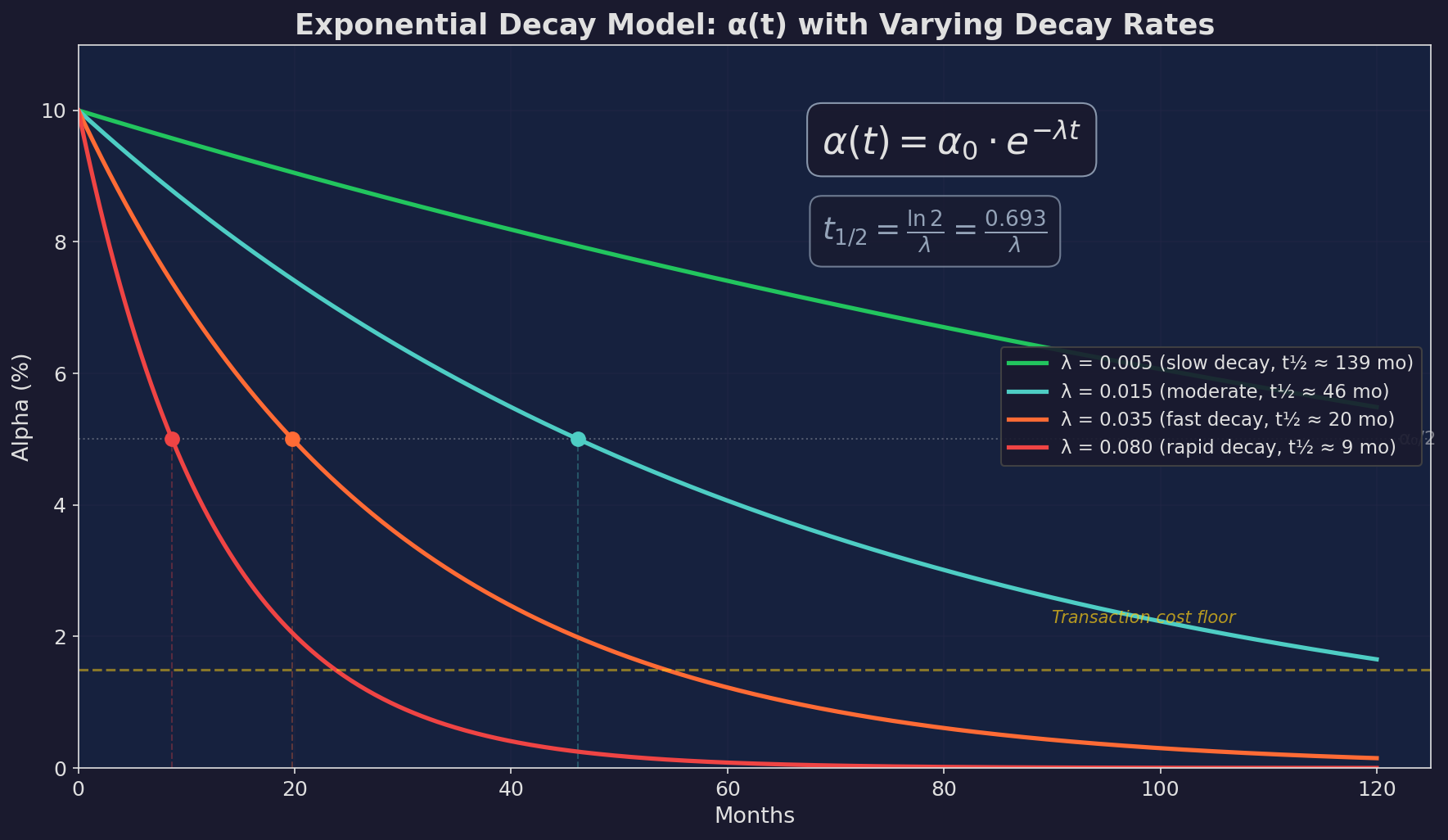
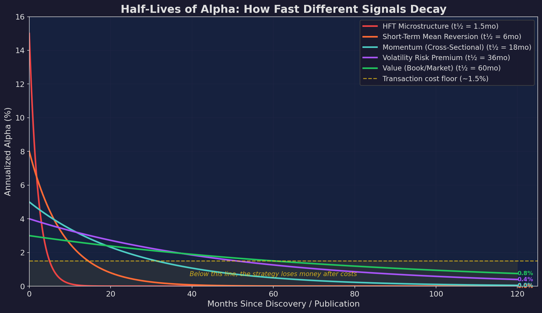
The critical insight is the transaction cost floor. Alpha doesn’t just decay toward zero — it becomes unprofitable once it drops below the cost of trading. For a typical retail strategy with 1-2% round-trip costs (spread + slippage + commissions), any signal with less than ~1.5% annualized alpha is actually a drag on returns.
This means the useful half-life is shorter than the mathematical half-life. A signal with α₀ = 5% and λ = 0.035 (t½ ≈ 20 months) hits the cost floor at:
1.5 = 5.0 · e^(-0.035·t)
ln(1.5/5.0) = -0.035·t
t = -ln(0.3) / 0.035
t ≈ 34.4 months
So the signal is mathematically “alive” for 20 months at half-strength, but only tradeable for about 34 months. After that, you’re paying more in costs than you’re earning in alpha.
Empirical Evidence: What the Research Shows
This isn’t just theory. There’s a growing body of academic evidence on post-publication decay.
The landmark study is McLean & Pontiff (2016), which examined 97 signals from academic finance journals. They found that post-publication returns declined by roughly 32% on average. But the averages mask huge variation — some signals lost nearly all their edge, while others appeared more resilient.
Here’s my synthesis of the evidence across signal types, pulling from McLean & Pontiff, Jacobs & Müller (2020), and AQR’s research:
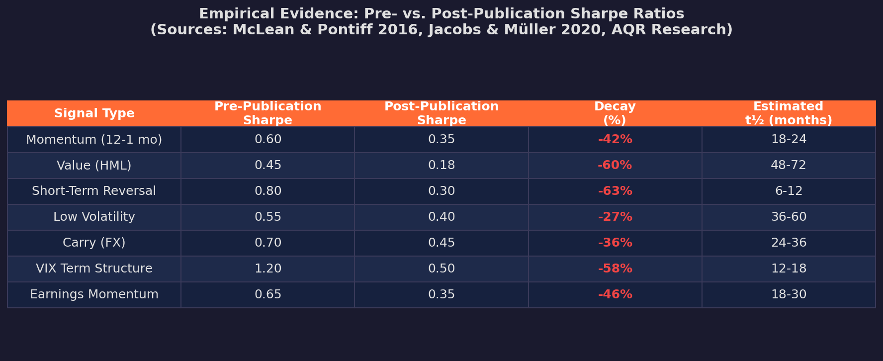
A few things jump out:
Short-term signals decay fastest. Short-term reversal lost 63% of its pre-publication Sharpe, with an estimated half-life of 6-12 months. This makes sense: short-term signals are easier to implement, so capital floods in quickly.
Structural risk premia are more resilient. Low volatility only lost 27% of its Sharpe. Why? Because the low-vol premium is partly driven by institutional constraints (benchmarking, tracking error budgets) that don’t go away just because you published a paper about them.
VIX term structure signals decayed fast. This one hit home for me. The VIX contango/backwardation trade was printing money in 2012-2017, but post-publication and post-”Volmageddon” (XIV blow-up in February 2018), the easy money evaporated. Estimated half-life: 12-18 months.
Why Strategies Decay: Three Mechanisms
The exponential decay model tells you that alpha erodes but not why. There are three distinct mechanisms, and understanding which one is killing your strategy determines what (if anything) you can do about it.

1. Crowding
The most intuitive mechanism. You find an edge. You trade it. Others find it too. Capital flows in. The signal gets arbitraged away.
The math of crowding follows a logistic diffusion model combined with a capacity constraint:
Participants(t) = P_max / (1 + e^(-k(t - t₀)))
α(t) = α₀ · (1 - Participants(t)/P_max)^γ
Where γ > 1 captures the nonlinear nature of crowding — the first few participants barely dent the alpha, but beyond some tipping point, returns collapse rapidly.
The speed of diffusion (k) depends on how the signal is discovered:
Channel                      Diffusion Speed (k)    Time to 50% Awareness
──────────────────────────────────────────────────────────────────────────
Academic journal                   0.08                  ~30 months
Quant blog / Substack              0.15                  ~18 months
FinTwit / Reddit                   0.35                  ~8 months
Retail brokerage feature            0.80                  ~3 months
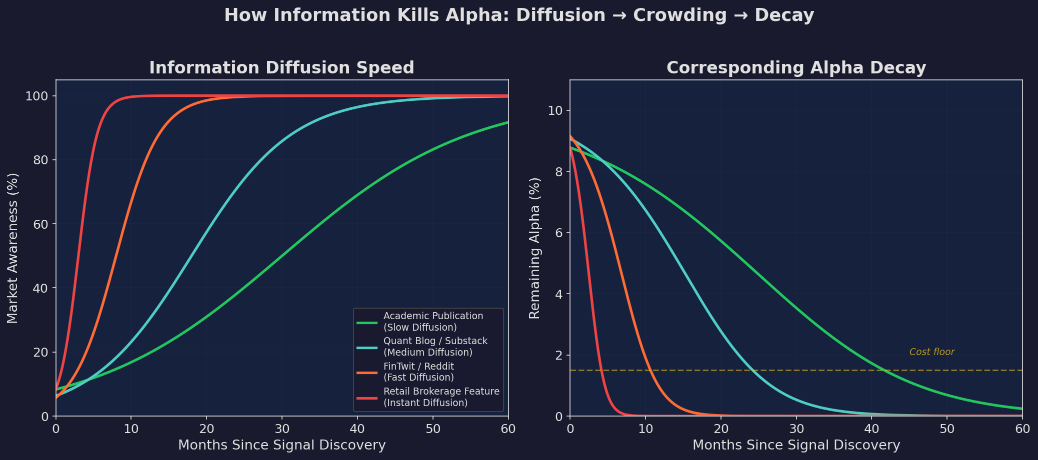
Left: how fast different channels spread awareness. Right: how the corresponding alpha decays. Faster diffusion → faster death.
This has an uncomfortable implication for what I’m doing with this Substack. Every time I write about a strategy, I’m contributing to its diffusion. The Recession Anxiety Index post probably didn’t move markets, but the principle applies: publicity accelerates decay.
The saving grace for retail quants is capacity. Large-cap momentum can absorb billions before degrading significantly. A micro-cap mean reversion strategy might only support $10M. If your strategy operates in a capacity-constrained niche, crowding is less of a threat — but so is your ability to scale.
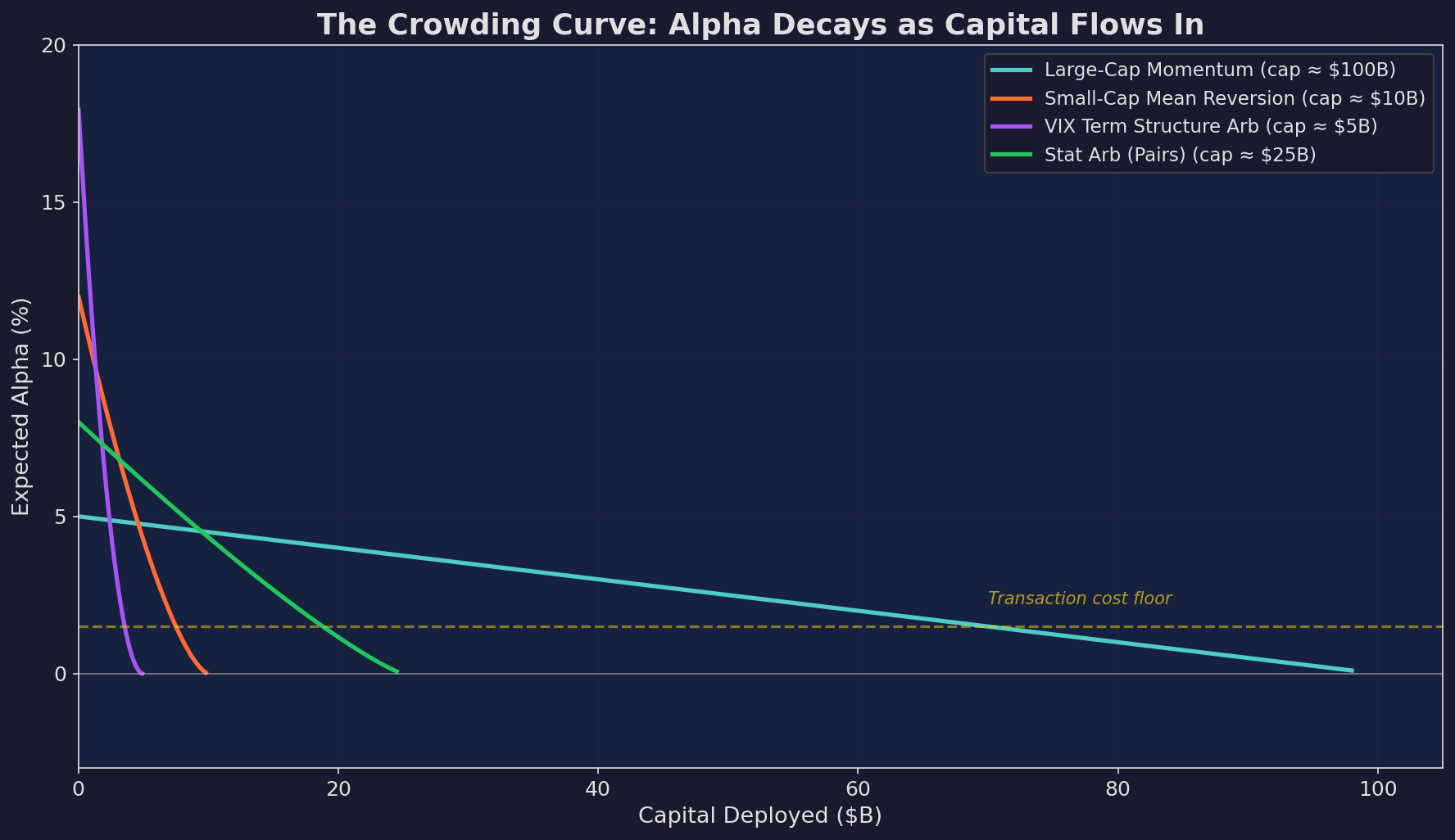
Different strategies have different capacity ceilings. VIX term structure arb hits zero alpha at ~$5B deployed. Large-cap momentum can absorb 20x that before breaking.
2. Regime Change
The market’s statistical properties shift. Correlations that were negative become positive. Volatility regimes flip. Interest rate environments change.
This is different from crowding because it’s not caused by other participants — it’s the world changing underneath your model.
I lived through this with the TLT hedge in V6. The strategy assumes negative stock/bond correlation during stress events. This relationship held beautifully from 2000 to 2021. Then 2022 happened: stocks and bonds fell together, and the hedge became a second source of losses.
Regime change produces a discontinuous decay rather than exponential. Alpha doesn’t gently decline — it drops off a cliff when the underlying relationship breaks.
The mathematical signature looks like:
α(t) = α_base + Δα · 𝟙[regime = favorable]Where 𝟙 is an indicator function that equals 1 when you’re in the right regime and 0 otherwise. The strategy doesn’t decay smoothly — it alternates between working and not working.
The danger is that regime changes look like drawdowns in real-time. You can’t distinguish “the strategy is temporarily losing money” from “the world has changed and the strategy is broken” without statistical tests, which is what Part 2 will cover.
3. Overfitting (The Signal Was Never Real)
The most humbling mechanism. The alpha wasn’t real in the first place. Your backtest found a pattern that existed in the historical data but was never a true market relationship.
This is what happened with my V5 ML model. It didn’t decay — it was never alive. The 6,000% return was an artifact of a data leak. When I fixed the leak, the “alpha” became a -28% loss.
Overfitting doesn’t follow an exponential decay curve. It follows a revelation curve: alpha appears stable in-sample, then drops abruptly when tested out of sample or deployed live.
The mathematical model:
In-sample:   α̂ = α_true + α_noise
Out-of-sample: α̂ = α_true
If α_true ≈ 0, then all the in-sample alpha was noise. Your backtest was measuring the noise component, which vanishes out of sample.
The number of parameters in your model is the best predictor of how much noise you’re capturing:
Expected noise alpha ≈ σ · √(k/n)Where k is the number of parameters, n is the number of observations, and σ is the noise level. V5 had hundreds of ML features. V6 has three parameters (momentum threshold, VIX thresholds, allocation weights). The expected noise alpha in V5 was orders of magnitude higher.
Putting It Together: The Half-Life Spectrum
Different signal types have inherently different half-lives, driven by their susceptibility to each of the three mechanisms:

HFT signals decay in weeks. Structural risk premia last years. Everything else is somewhere in between.
The key takeaway for my own work:
V6 is a momentum + volatility regime strategy. Cross-sectional momentum has an estimated half-life of 18-24 months. The VIX regime component is harder to classify — it’s partly a structural risk premium (volatility sells off during calm periods) and partly a timing signal (which decays faster).
My best estimate for V6’s alpha half-life: 18-36 months, assuming the stock/bond correlation relationship holds and the momentum signal continues to work.
That’s not forever. It means I need to be actively monitoring for decay and preparing to adapt — which is exactly what Parts 2 and 3 of this series will cover.
What This Means for Retail Quants
A few practical implications:
1. Simplicity extends half-life. Complex strategies overfit more and decay faster. V6 works partly because it’s simple. Three inputs, one decision tree, one hedge. There’s less to break.
2. Structural edges decay slower than statistical edges. The TLT flight-to-quality trade works because of institutional behavior (pension funds, central banks) not because of a statistical anomaly. That’s harder to arbitrage away. Look for strategies where the reason the edge exists is durable.
3. Publication accelerates decay. Every time someone writes about a strategy on Substack or FinTwit, the clock speeds up. This creates an ironic tension for people like me who build in public. The act of sharing knowledge erodes the edge being shared. On the other hand, you keep testing and building new strategies, so that’s an advantage. But you’ll notice I don’t share everything (e.g., my Dual Allocator code) — and that’s with good reason.
4. You need a monitoring framework. If alpha has a half-life, you need instruments to measure it in real-time. “Trust the backtest” is not a monitoring framework. Part 2 will look at building one.
Up Next
Part 2: Detecting Decay in Real-Time — CUSUM tests, Page’s test, Bayesian changepoint detection, and building a dashboard that tells you when your strategy is dying.
Remember: Alpha is never guaranteed. And the backtest is a liar until proven otherwise.
These posts are about methodology, not recommendations. If you find errors in my math, let me know — I’ve built an entire series around discovering my own mistakes, so one more won’t hurt.
The material presented in Math & Markets is for informational purposes only. It does not constitute investment or financial advice.