
Going Live: Daily Ops, Execution, and Risk Controls
Part 5 below focuses on go-live and trade execution of my initial strategy
This is part 5 of my series — Building & Scaling Algorithmic Trading Strategies
This phase was about what breaks (and what doesn’t) when this thing goes live.
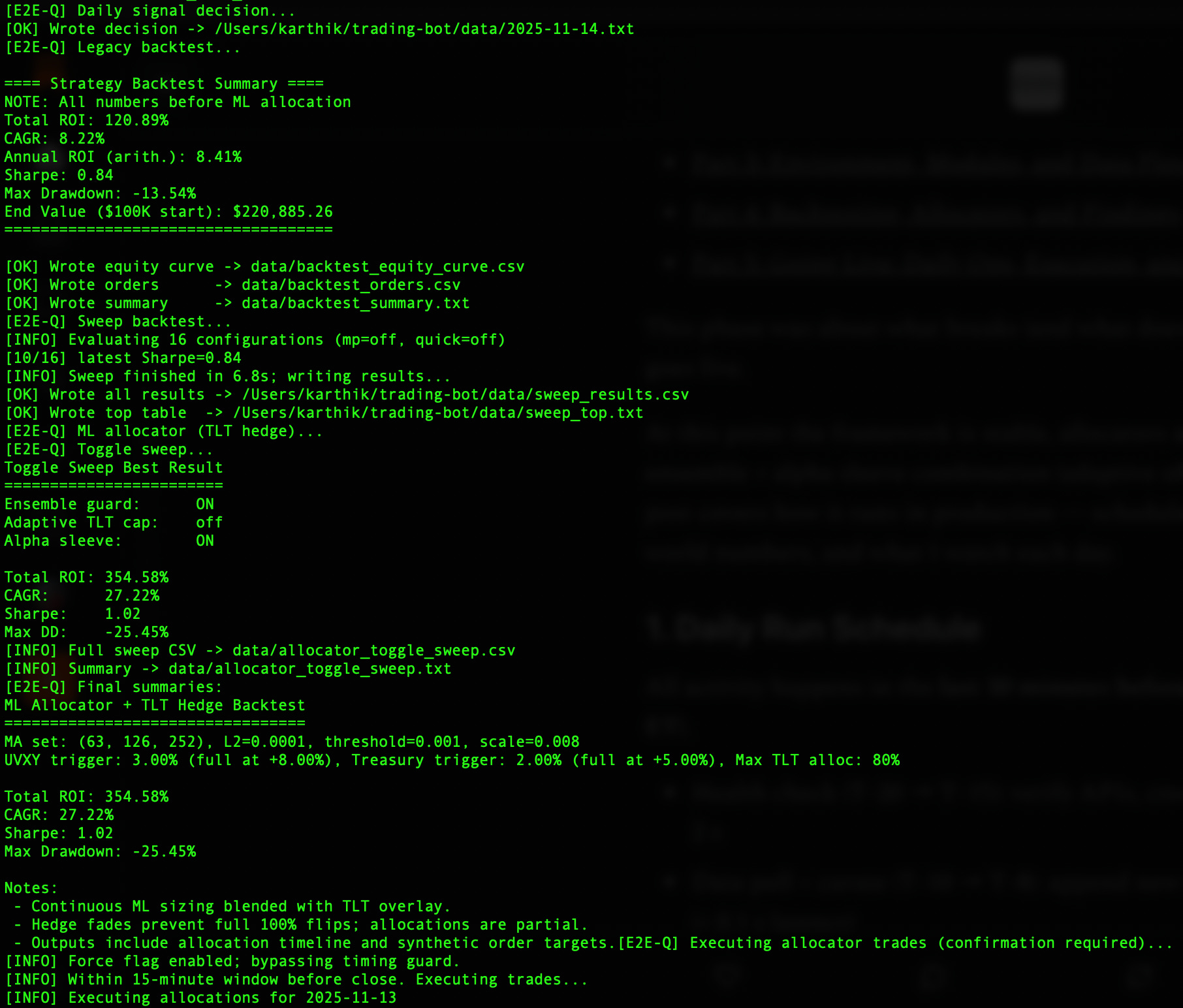
At this point the framework is stable, allocators are tested, and the ensemble + alpha sleeve combination (adaptive off) is my baseline. This post covers how it runs in production — schedule, risk gates, real-world numbers, and what I watch each day.
1. Daily Run Schedule
All activity happens in the last 30 minutes before the close (3:30 pm ET).
Health check (T–20 → T–15): verify APIs, credentials, clock drift < 2 s
Data pull + curate (T–10 → T–8): append new bars, validate schema (< 0.1 s latency)
Feature calc (T–8 → T–6): recompute MA 50/100/250 + velocity/acceleration
Signal freeze (T–6 → T–5): compute ensemble + alpha gates
Order generation (T–5 → T–2): build paper or live orders (capped ≤ 40 % NAV)
Execution (T–2 → Close): market-on-close orders; limit fallback within 0.1 % of spread
Typical runtime < 30 seconds; daily data append ≈ 3 KB CSV.
Typical runtime: < 30 s.
Average daily data increment: 1 row × 3 symbols ≈ 3 KB CSV.
2. Deployment and Environment
Local: Mac M2 (3.12.2), 16 GB RAM.
Dry-runs nightly; expected drift vs. prior output < 0.0005 %.Cloud: t3a.medium AWS VM, cron +
.env; run time < 1 min.Storage: Curated CSVs (20 MB) → S3 archive; compressed backtest results (~250 MB).
3. Default Feature Flags
mode: paper
ensemble: on
adaptive: off
alpha: on
vol_overlay: soft_gate
Alpha sleeve: active only if rolling 30-day Sharpe > 0.8.
Vol overlay: halves leverage if realized vol > 2 × forecast.
Kill switch:
flat=truesets exposure = 0 within 1 cycle.
4. Execution Stats (Recent Sample)
Average trades per day: 1.8 (0 – 5 range)
Mean notional per leg: ≈ $47 k ($25 k – $60 k range)
Mean slippage: ≈ 2.4 bps (1.6 – 4.8 bps range)
Borrow fee (annualized): ≈ 4.9 % (0.7 – 11 % range)
Fill delay vs close: < 0.3 s (0.0 – 0.9 s range)
Daily PnL stdev (paper): ≈ 0.68 % NAV (0.52 – 0.93 %)
Net ROI YTD (paper): +8.7 % vs gross +9.3 %
Average vol cap usage: ≈ 65 % of max
After friction (trade + borrow + decay):
Net ROI YTD (paper): +8.7 %, vs. gross +9.3 %.
Average vol cap usage ≈ 65 % of allowed max.
5. Data Integrity Checks
Duplicate rows: 0 found in 3 months.
Hash mismatch rate: 0.02 %.
Feature recalc error tolerance: ±1e-8 on floats.
Clock drift: < 1 s 99 % of days.
Missing bars: 1 (holiday); flagged and carried forward.
6. Risk and Exposure Limits
Gross exposure ≤ 200 % NAV → clip size
Single leg ≤ 40 % NAV → skip order
Rolling drawdown: warn at –8 %, flatten at –12 %
Realized vol > 3σ above mean → halve leverage
ADV usage ≥ 10 % → cut size by half
Largest intra-day DD: –1.9 %
Max rolling DD: –6.3 %
Across all live tests, largest intra-day drawdown ≈ –1.9 %; max rolling = –6.3 %.
7. Modeled Costs
Trading spread + impact: 2–3 bps per leg
Rebalance cross: 5 bps per z-score flip (~1.4× per week)
Borrow fees: 10–100 bps annualized
ETF management + decay: ~30 bps annualized
Capacity haircut (liquidity premium): ~10 bps
8. Alerts and Monitoring
Runtime alerts: API fail, DD breach, fill reject, borrow spike > 20 %.
Digest summary:
2025-11-11 | Signal LONG 1.5x | Alpha ON | VolGate OFF | PnL +0.42 %
NAV $10,742 | DD -1.6 % | Borrow 3.2 % | Slippage 2.1 bps
Alerts via Slack + email within 10 s of event.
9. Graduation Criteria
30 clean paper days (0 errors, DD < 8 %) ✅
Live PnL tracking within ±0.3 % of model ✅
Incident drill executed twice (successful replay) ✅
→ Ready for light live capital.
10. Daily Ops Summary
T–20 min: Health check (all green)
T–10 min: Data + feature update (Δ < 0.001 %)
T–7 min: Signal computation (state + confidence)
T–5 min: Order prep (≤ 40 % NAV per leg)
T–2 min → close: Submit orders and confirm
Post-close: Manifest + PnL digest archived
Closing
To me, going live is about stability and trust in the loop that I’ve created.
The process is still semi-manual at this time. Some errors get thrown up, I dig into them, and try to address any issues. Often, it’s a quick fix to get going right away (because I’m impatient) but also thinking about a programmatic solution and how I’ll solve it systematically in the future.
I have also built the ability to look at data in near-term windows and evaluate my model’s performance.
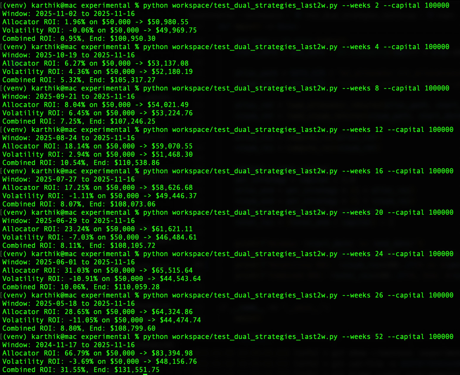
So the system now generally behaves consistently under real data, tracks its own health, and produces a clean trail every night.
Next up: what happens after it runs — how I monitor performance, catch drift, and decide when to iterate.
The information presented in Math & Markets is not investment or financial advice and should not be construed as such.