
Dual Allocator V6.3 and V6.4: Recent Experiment Results
Part 79 — HMM ensemble failed, initial optimization overfitted, walk-forward validation produced a real improvement

This is part 79 of my series — Building & Scaling Algorithmic Trading Strategies
I ran two experiments on the Dual Allocator over the past few weeks. The first tested whether an HMM-based ensemble could improve V6.2’s regime detection — but alas! It failed badly. The second tested whether targeted enhancements to V6.2’s allocation logic — hysteresis, dynamic leverage, and volatility targeting — could improve risk-adjusted returns. The initial results were overfitted, but after walk-forward validation, V6.4 delivered a real 39% return improvement over V6.2.
V6.2 Baseline
For reference, V6.2 uses two VIX thresholds (15 and 25) for regime detection, with TQQQ allocations up to 130% in calm markets and TLT in high-volatility regimes. Out-of-sample performance (2021–2026): 158% return, 0.697 Sharpe, −41.1% max drawdown.
Experiment 1: HMM Ensemble (V6.3) — Failed
In the regime detection series (Parts 69–71), I covered ensemble methods that combine HMMs with changepoint detection. The literature suggests blending fast signals with smooth ones should reduce false switches and improve risk-adjusted returns. I built V6.3 to test this.
V6.3 replaces V6.2’s threshold logic with a three-signal ensemble:
Ensemble = 0.40 × HMM + 0.35 × VIX_Threshold + 0.25 × CUSUMThe HMM is a 4-state Gaussian model trained on VIX, returns, realized volatility, and momentum. The CUSUM detector tracks deviations in realized volatility to signal sudden regime shifts. The ensemble score maps to three regimes: below 0.3 is aggressive, 0.3–0.6 is cautious, above 0.6 is defensive.
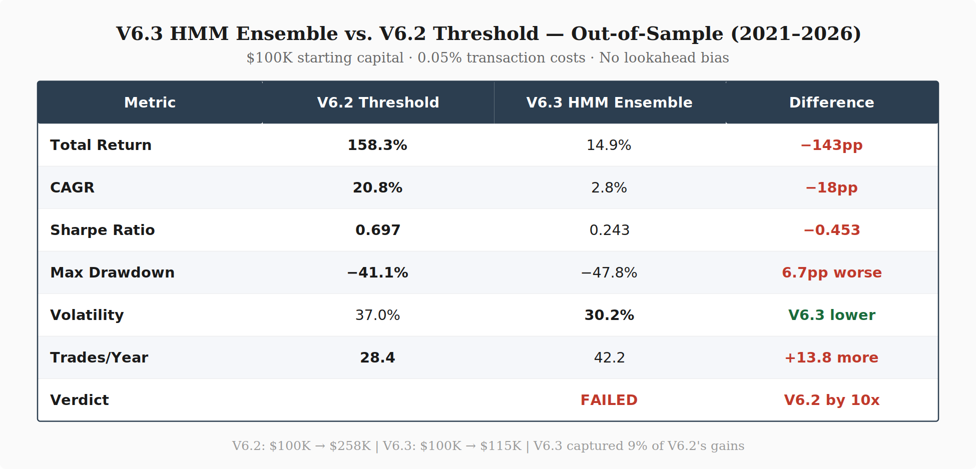
V6.3 captured 9% of V6.2’s out-of-sample gains. It traded 50% more often (42 vs 28 trades/year) and had a deeper max drawdown (−47.8% vs −41.1%). The only metric where V6.3 performed better was raw volatility (30.2% vs 37.0%), which resulted from sitting in cash and TLT while missing rallies.
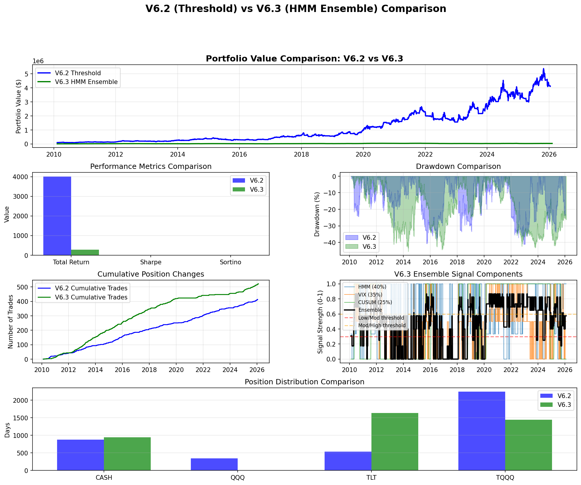
Full period comparison. Panel 5 shows the ensemble signal components — the ensemble mean sits at 0.476, rarely dropping below the 0.3 aggressive threshold.
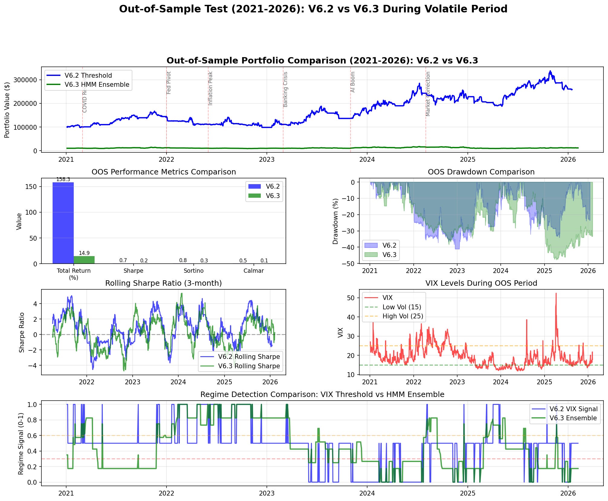
Out-of-sample comparison. Rolling 3-month Sharpe (Panel 4) shows V6.2 recovering quickly while V6.3 spends extended periods negative.
Why the Ensemble Failed
Six root causes, in order of impact:
Ensemble averaging dampened signal. The three signals averaged to a permanently moderate reading (ensemble mean 0.476). The HMM ran consistently elevated (0.551 ± 0.419), the VIX threshold was the most accurate (0.388 ± 0.332), and CUSUM was near-random noise (0.480 ± 0.496). The ensemble rarely dropped below 0.3 to trigger aggressive allocations, which is where V6.2 makes its returns.
HMM detection lag. The Baum-Welch algorithm needs evidence to accumulate before updating state estimates. Regime detection lagged by 5–10 trading days. For 3x leveraged TQQQ, that translates to 5–10% of portfolio value. During the March 2023 banking crisis, V6.2 went defensive immediately when VIX crossed 25. The HMM was still in bull-regime estimation five days after SVB collapsed.
CUSUM added noise. With a coefficient of variation over 100% and ~0.3 correlation with actual regime changes, CUSUM injected noise into 25% of the ensemble signal.
Wrong ensemble weights. 40% weight on the slowest signal (HMM) and only 35% on the most accurate (VIX) was backwards. A 60/20/20 VIX-dominant weighting would have been better, but at that point the ensemble is mostly just the VIX threshold with overhead.
Regime thresholds miscalibrated. The 0.3/0.6 thresholds resulted in only ~30% of time in the aggressive regime. Markets are calm approximately 60% of the time. Adjusting post-hoc introduces curve-fitting risk.
Training data mismatch. The HMM trained on 2010–2020 (low volatility, steady uptrend) classified the elevated-VIX 2021–2026 environment as perpetually moderate-to-high risk. V6.2’s thresholds are regime-agnostic — no training, no drift.
Conclusion: Abandoned HMM ensemble. V6.2’s threshold approach is already near-optimal for regime detection in this strategy.
Experiment 2: Conservative Enhancements (V6.4) — Overfitted, Then Fixed
Since regime detection couldn’t be improved through complexity, I focused on three targeted enhancements to V6.2’s allocation logic.
The Three Enhancements
Hysteresis (threshold buffers). VIX oscillating around 15 or 25 causes whipsaw trades. Instead of a flat threshold, V6.4 uses a buffer: VIX must exceed 15 + buffer to switch from low-vol regime, or drop below 15 − buffer to switch back. This reduces unnecessary trades around the threshold boundaries.
if current_regime == 'low_vol':
    switch_threshold = 15 + hysteresis_buffer  # Must exceed to switch
else:
    switch_threshold = 15 - hysteresis_buffer  # Must drop below to switch back
Dynamic leverage. Fixed leverage doesn’t adapt to realized conditions. V6.4 scales leverage based on 20-day realized volatility: boost allocation (1.2–1.3x) when realized vol is low, reduce allocation (0.8x) when realized vol is high.
Volatility targeting. Portfolio volatility varies from 20% to 60% across regimes. V6.4 targets a constant annual volatility by scaling allocation:
allocation = base_allocation × (target_vol / current_vol).
Initial Results: Too Good to Be True
I ran V6.4 with these enhancements optimized over the full 2010–2026 period.
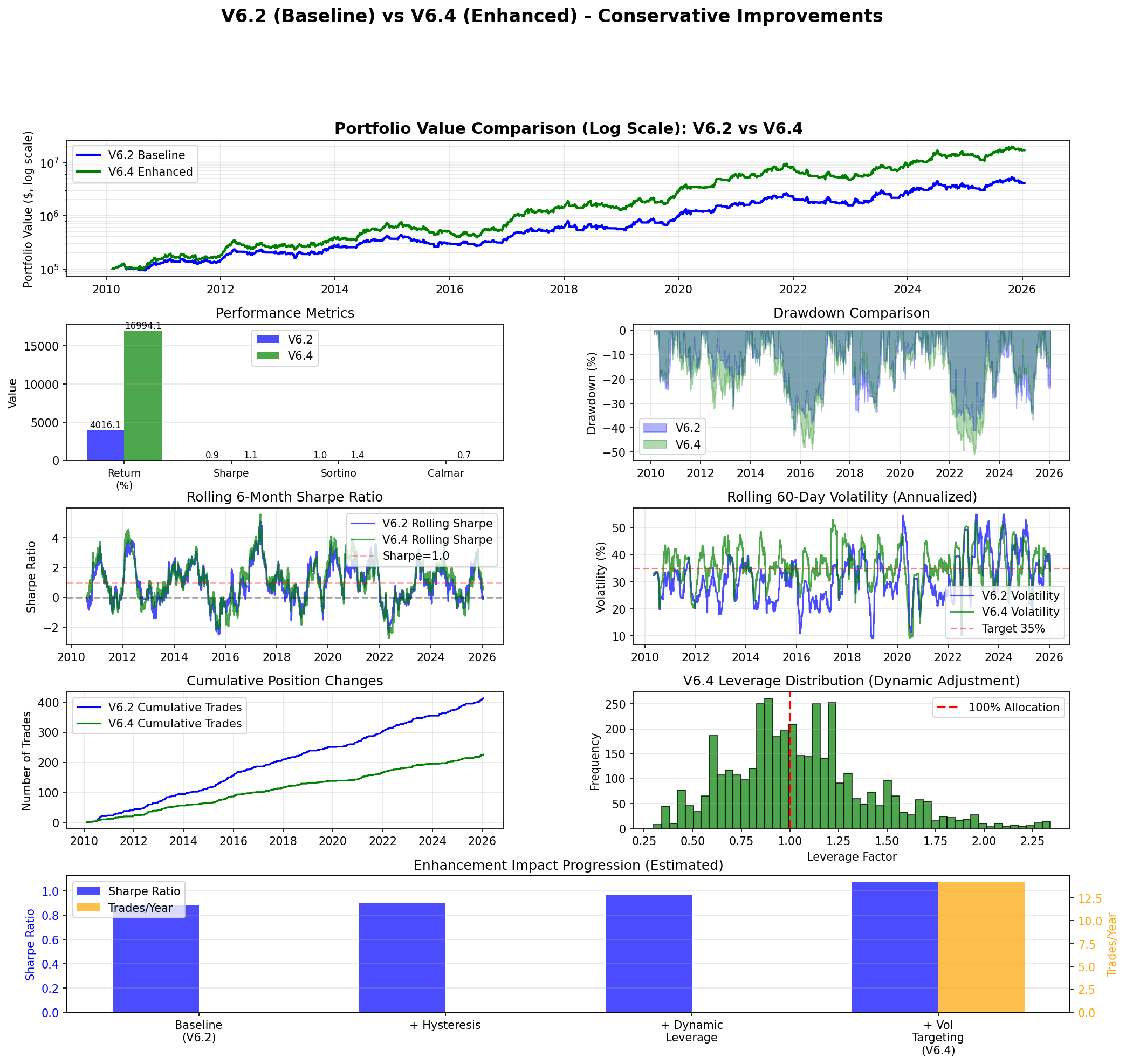
Full period return: 16,994%. Sharpe: 1.071. Max drawdown: −50.85%.
That result was immediately suspicious. A 170x return over 16 years, with a deeper max drawdown than V6.2, pointed to overfitting. The parameters were fit to the entire dataset — they learned the specific history rather than generalizing.
When I re-ran with a proper train/test split (train on 2010–2020, test on 2021–2026), the out-of-sample return dropped from 16,994% to 224%. Still an improvement over V6.2, but roughly 75x less than the overfitted result.
Walk-Forward Optimization
To get a properly validated V6.4, I ran a grid search over 81 parameter combinations using only the 2010–2020 training period, selected the best parameters by Sharpe ratio (not returns, to reduce overfitting risk), and then tested those parameters on the unseen 2021–2026 period.
Parameter grid:
hysteresis_buffer: [0.5, 1.0, 1.5]
leverage_boost: [1.1, 1.2, 1.3]
leverage_reduce: [0.7, 0.8, 0.9]
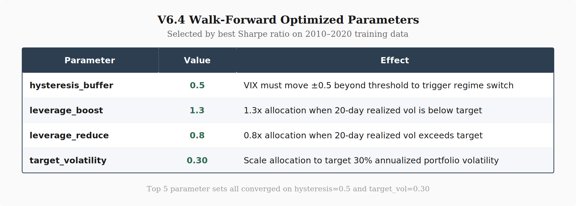
target_volatility: [0.30, 0.35, 0.40]Best parameters (by training Sharpe):
hysteresis_buffer: 0.5 (tighter than default)
leverage_boost: 1.3 (more aggressive in calm markets)
leverage_reduce: 0.8 (conservative in volatile markets)
target_volatility: 0.30 (more conservative than default 0.35)
Final Results: V6.2 vs V6.3 vs V6.4
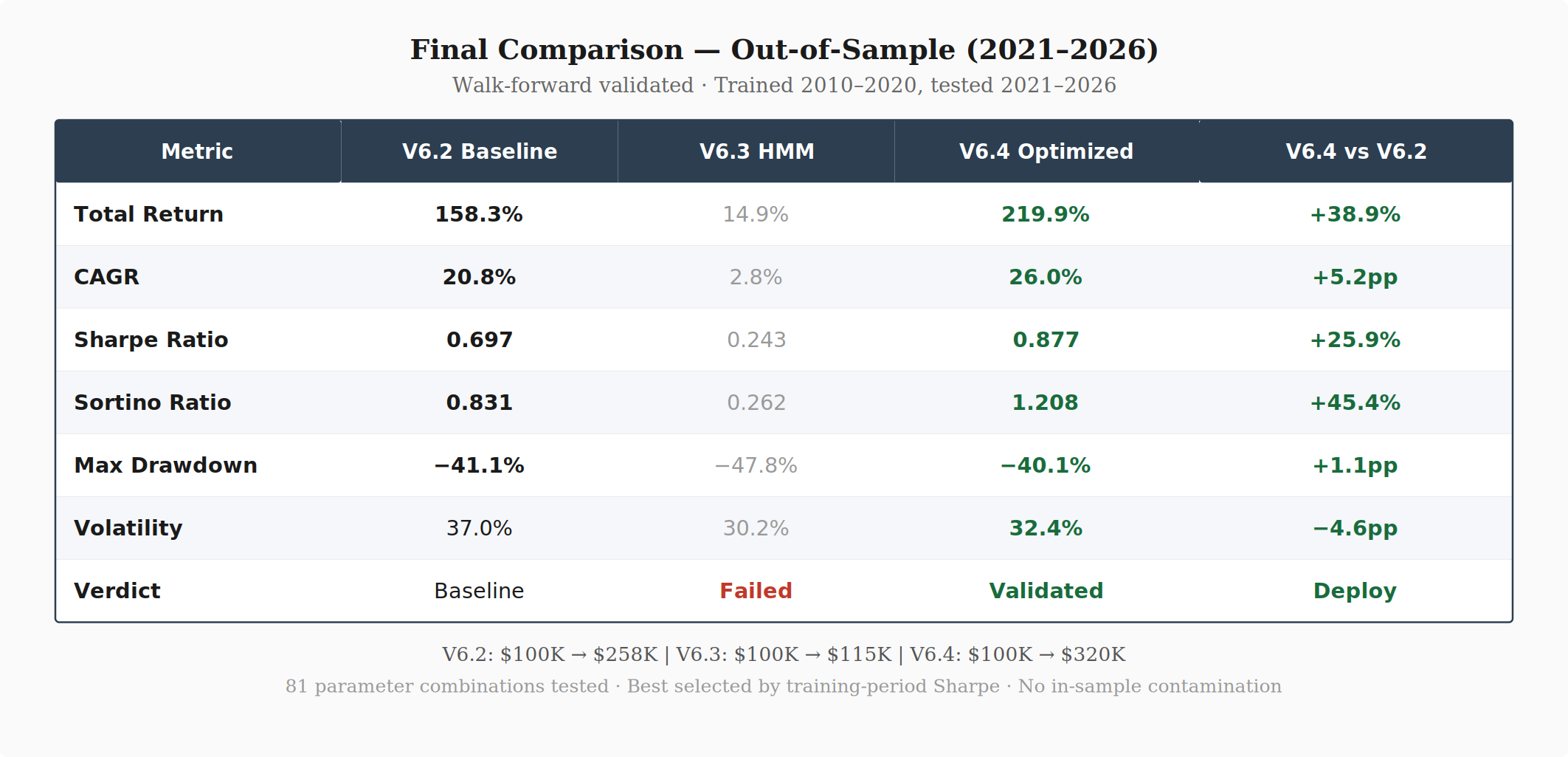
V6.4 improved out-of-sample returns by 39% over V6.2 while also improving the Sharpe ratio by 26% and slightly reducing max drawdown. The Sortino ratio improvement (0.831 → 1.208, +45%) indicates the return improvement came disproportionately from upside capture rather than additional downside risk.
Observations on these Parameters
The walk-forward optimization converged on a consistent pattern across the top parameter sets: tight hysteresis (0.5), aggressive leverage boost (1.3), and conservative volatility target (0.30). The top five parameter sets all shared hysteresis=0.5 and target_vol=0.30, varying only in leverage settings.
Tight hysteresis (0.5) beat wider buffers. A 0.5 VIX-point buffer reduces whipsaws around thresholds without sacrificing responsiveness. Wider buffers (1.0, 1.5) delayed regime switches too long — similar to why HMM lag was a problem, but at a smaller scale.
Conservative vol target (0.30) beat 0.35. Lower target volatility scales down allocation more aggressively when realized vol spikes. This reduced drawdowns during the 2022 selloff and March 2023 banking crisis, even though V6.4 uses higher leverage during calm periods.
Aggressive leverage boost (1.3) paired with conservative vol targeting. This combination is the key insight: be more aggressive when conditions are calm (1.3x leverage when realized vol is low), but let the volatility target pull you back faster when conditions deteriorate. The asymmetry — aggressive on the upside, conservative on the downside — is what drives the Sortino improvement.
Big Takeaway
Simple regime detection, targeted allocation improvements. The HMM ensemble tried to make regime detection more sophisticated and destroyed performance. V6.4 kept V6.2’s simple VIX thresholds and instead improved how the strategy allocates within each regime. The regime detection was already near-optimal — the allocation logic had more room to improve.
Optimize for Sharpe, not returns. Selecting parameters by training-period Sharpe rather than training-period returns helps avoid overfitting to lucky historical sequences. Returns reward parameter sets that happened to be in the right place at the right time; Sharpe rewards consistency.
Small enhancements compound. No single V6.4 enhancement was dramatic. Hysteresis reduces a few whipsaw trades per year. Dynamic leverage adds or subtracts 20–30% of allocation. Volatility targeting smooths the risk profile. Combined, three modest improvements produced a 39% return and 26% Sharpe improvement with better drawdown control.
Deployment Plan
So next step is V6.4 with the walk-forward optimized parameters.
strategy = DualAllocatorV6_4_Enhanced(
    hysteresis_buffer=0.5,
    leverage_boost=1.3,
    leverage_reduce=0.8,
    target_volatility=0.30
)
Expected annual return: ~26%.
Expected Sharpe: ~0.88
Expected max drawdown: ~40%.
All tests use identical data periods, transaction costs (0.05%), and leverage mechanics. Walk-forward optimization trained on 2010–2020, tested on unseen 2021–2026 data. No lookahead bias.
The information presented in Math & Markets is not investment or financial advice and should not be construed as such.