Does Lower Delta Mean Lower Expected Value? The Retail Effect on Options Pricing

Part 49 discusses fat tails, volatility surfaces, and why delta doesn't determine expected value

This is part 49 of my series — Building & Scaling Algorithmic Trading Strategies

---

A recent discussion on the r/thetagang subreddit raised an interesting question that gets to the heart of options pricing theory versus market reality. After a rough couple of days for tech, someone asked how traders who sold 0.3 delta puts were holding up. The responses ranged from pragmatic (”I stick to 0.15 delta or lower”) to theoretical (”the lower the delta you go, the lower the EV”).

That theoretical claim deserves a closer look, because the math is more nuanced than it first appears, and the rise of retail options trading has introduced structural changes that affect how we should think about protection and hedges.

What Delta Actually Measures

Delta is often described as the probability that an option expires in the money, but this is a convenient approximation rather than a precise definition. Technically, delta is a rate sensitivity: it tells you how much an option’s price changes for a $1 move in the underlying asset. Under the Black-Scholes model, delta happens to approximate the risk-neutral probability of expiring ITM, but this relationship depends on assumptions that don’t hold perfectly in real markets.

The key assumption is that stock returns are lognormally distributed, which implies that log returns follow a normal (Gaussian) distribution. Under this framework, if you sell a 0.1 delta put, the model says there’s roughly a 10% chance the underlying drops enough to put you in trouble. The argument that “lower delta means lower EV” follows from this logic: as you move further out of the money, you’re selling increasingly unlikely outcomes for smaller premiums.

But real return distributions aren’t normal. They exhibit what statisticians call leptokurtosis, or fat tails, meaning extreme moves happen more frequently than a normal distribution would predict. The 2020 COVID crash, the 2008 financial crisis, and countless flash crashes all represent tail events that occurred with frequencies far exceeding what Gaussian models suggest.

The Math Behind Delta and Probability

To understand why the “lower delta = lower EV” claim breaks down, we need to look at how delta is actually calculated and what assumptions it encodes.

In the Black-Scholes framework, delta for a call option is:

Δ_call = N(d₁)

where N(·) is the cumulative normal distribution function, and d₁ is calculated as:

d₁ = [ln(S/K) + (r + σ²/2)T] / (σ√T)

Here S is the current stock price, K is the strike price, r is the risk-free rate, σ is volatility, and T is time to expiration. For puts, delta is N(d₁) - 1, which gives a negative value.

The probability of expiring in the money under Black-Scholes is actually N(d₂), not N(d₁), where:

d₂ = d₁ - σ√T

The difference between d₁ and d₂ is the volatility adjustment term σ√T. This matters because when people say “a 0.1 delta put has a 10% chance of expiring ITM,” they’re conflating delta with the ITM probability — which is already an approximation, and one that assumes constant volatility and lognormal returns.

Why Lognormal Assumptions Matter

Under Black-Scholes, stock prices follow geometric Brownian motion:

dS = μS dt + σS dW

This implies that log returns are normally distributed:

ln(S_T / S_0) ~ Normal((μ - σ²/2)T, σ²T)

A normal distribution has kurtosis of exactly 3. Real equity returns typically show excess kurtosis of 1-5 or more, meaning kurtosis values of 4-8. This is leptokurtosis — the distribution has fatter tails and a sharper peak than normal.

To put numbers on this: under a normal distribution, a 4-sigma event (roughly a 0.003% probability) should happen about once every 126 years of daily returns. In actual equity markets, 4-sigma daily moves happen every few years. The October 1987 crash was a 20+ sigma event under normal assumptions — essentially impossible, yet it happened.

How Implied Volatility Corrects for This

The market’s solution is to vary implied volatility by strike. If we invert the Black-Scholes formula to solve for implied volatility given market prices, we get:

σ_implied(K) = BSInverse(C_market, S, K, r, T)

When σ_implied increases as K moves away from S (the volatility smile), the market is effectively saying: “the Black-Scholes model with constant volatility underprices these options, so we’ll plug in a higher volatility to get the right price.”

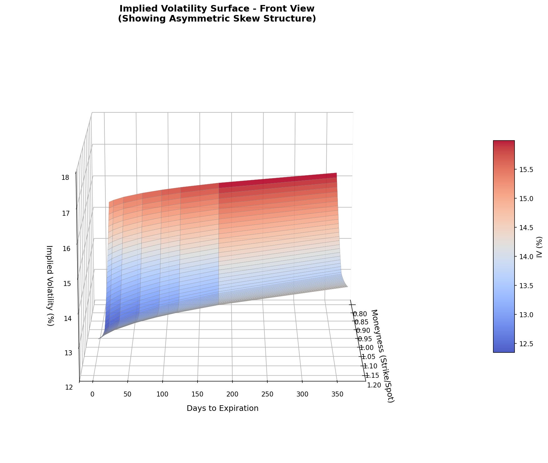
For equity indices, the smile is asymmetric — a smirk — with much higher IV on downside strikes:

σ_implied(K < S) >> σ_implied(K = S) > σ_implied(K > S)

This asymmetry reflects crash risk: the market assigns higher probability to large down moves than to equivalent up moves, which makes sense given the empirical distribution of equity returns.

Expected Value Is Not Monotonic in Delta

The expected value of selling an option depends on the relationship between what you collect (the premium, which reflects implied volatility) and what you expect to pay out (which depends on realized volatility and the true return distribution).

E[P&L] = Premium_collected - E[Payout]
       = f(σ_implied) - g(σ_realized, true_distribution)

If implied volatility perfectly reflected the true distribution, expected P&L would be zero for all strikes (ignoring risk premia). But it doesn’t — and the gap between implied and realized varies by strike.

The volatility risk premium (VRP) is typically defined as:

VRP = σ_implied - σ_realized

Historically, VRP has been positive on average (implied > realized), which is why selling options has been profitable. But the magnitude of VRP varies by strike and maturity. Deep OTM puts often have higher implied volatility but may also have higher “true” probability of payout than the lognormal model suggests — so the VRP at that strike could be smaller, zero, or even negative.

This is why you cannot read expected value from delta alone. A 0.05 delta put might have:

• Higher IV than a 0.20 delta put (due to skew)

• Similar or higher true probability of payout (due to fat tails)

• Lower, equal, or higher expected P&L depending on which effect dominates

The relationship is empirical, not mechanical.

The Volatility Surface Tells a Different Story

If markets were truly lognormal, implied volatility would be constant across all strike prices for a given expiration. Instead, we observe what’s called a volatility smile or skew: implied volatility increases as you move away from the current price, particularly on the downside for equity options.

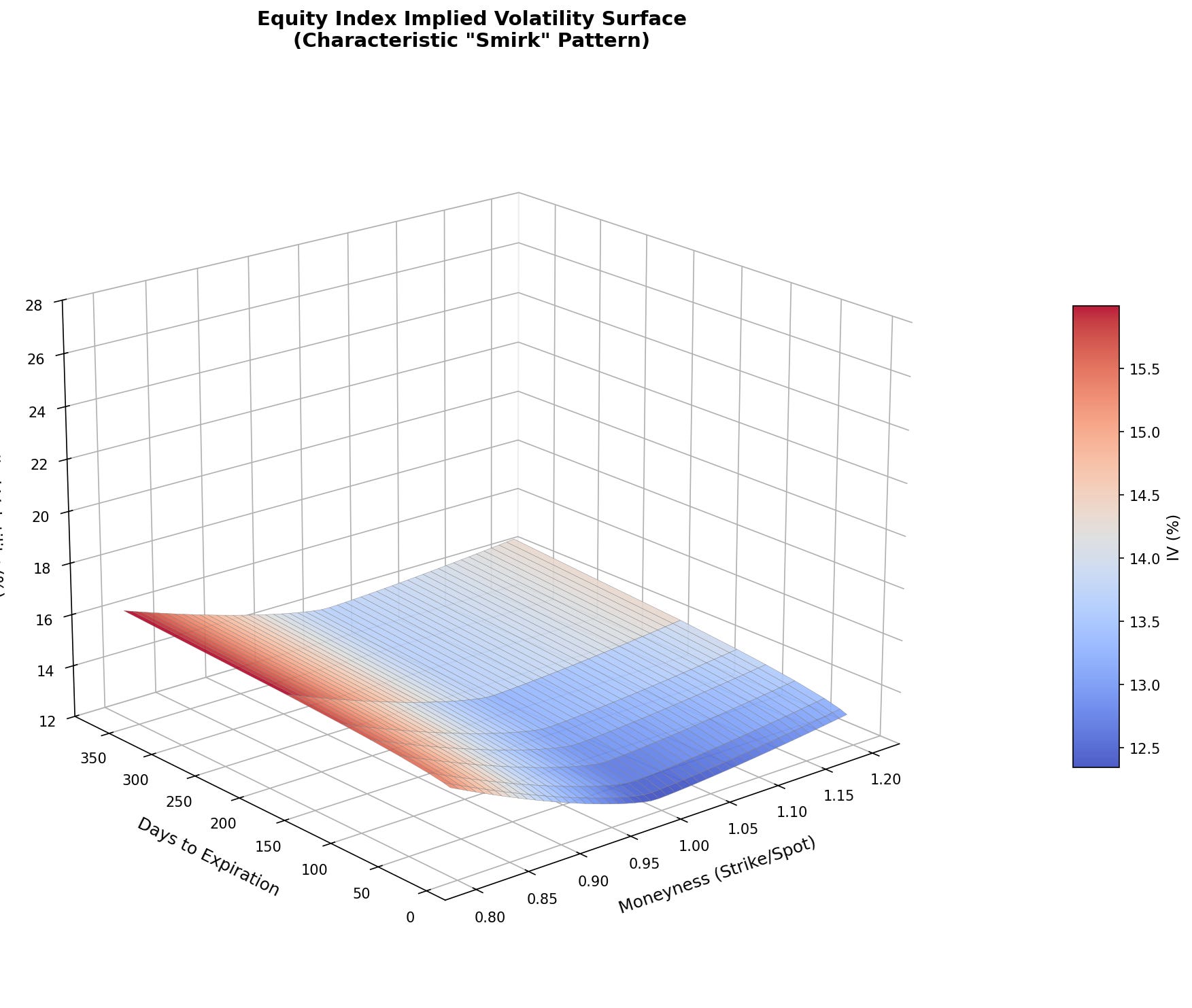
This skew exists precisely because market participants recognize fat tails and reprice accordingly. Deep out-of-the-money puts often carry higher implied volatility than at-the-money options, which reflects the market’s collective judgment that crash probabilities exceed what a lognormal model would suggest. In effect, the volatility surface is the market’s attempt to correct for the inadequacy of the normal distribution assumption.

The practical implication is that expected value across strikes is not monotonic. Some low-delta options are overpriced relative to their true risk (offering positive EV to sellers), while others are underpriced (negative EV to sellers). The relationship depends on where the volatility risk premium — the gap between implied and realized volatility — is concentrated, and that varies by strike, maturity, and market conditions.

Enter the Retail Trader

Here’s where the discussion took an interesting turn. One commenter argued that while markets historically priced fat tails via the volatility smile, the massive influx of retail traders into options markets has changed the shape of this curve.

The classic volatility smile — elevated IV on both wings — has evolved into more of a volatility smirk in many markets. The explanation is structural: retail traders disproportionately sell options, particularly on the wings, and this selling pressure suppresses premiums on low-delta strikes relative to where they would be in a market dominated by institutional hedgers.

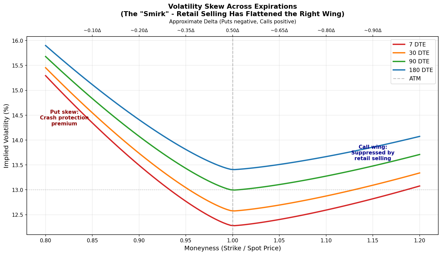
The volatility risk premium (VRP) — historically a reliable source of returns for options sellers — has been shrinking as more participants compete to harvest it. This compression is not uniform across strikes; it tends to be most pronounced at popular strikes where retail flow concentrates. If you’re selling the same 0.1 delta weekly puts that thousands of other retail traders are selling, you may be competing away the edge that strategy once had.

The empirical evidence here is mixed but suggestive. Studies of options returns show that the relationship between moneyness and expected returns is complex: for some equities, deep OTM calls have negative expected returns after adjusting for the VRP, while near-ATM short options can still offer meaningful positive premia. The shape is driven by the interplay of volatility risk premium, skew, and retail flow, not by delta alone.

What This Means for Protection Strategies

One trader in the discussion mentioned a specific hedge structure: selling one 0.1 delta put and buying seven 0.01 delta puts at 60-100 DTE. The idea is that in a flash crash scenario, the 0.01 delta puts experience explosive gamma and IV expansion, potentially multiplying in value enough to offset losses on the short 0.1 delta and then some.

This strategy is essentially a leveraged bet on two things happening simultaneously during a sharp, fast decline: massive re-steepening of downside skew (deep OTM IV exploding relative to near-OTM), and gamma transitioning from nearly zero on the 0.01 delta line to substantial as the underlying trades down through those strikes.

Does the retail-driven suppression of wing premiums undermine this hedge? The answer is nuanced. On one hand, if the 0.01 delta puts are cheaper than they “should” be given true crash probabilities, the hedge is actually more attractive than it would otherwise be. You’re buying underpriced lottery tickets. On the other hand, if the 0.1 delta put you’re selling is also suppressed, your premium income is lower, and your ratio may need to shift to maintain the same risk profile.

The deeper issue is that the hedge’s effectiveness depends on market structure during the crash itself. In a true flash crash, the question is not just what the theoretical value of your deep OTM puts becomes, but whether you can actually realize that value given liquidity conditions, bid-ask spreads, and market maker behavior. The March 2020 experience showed that even supposedly liquid options can gap in unpredictable ways during stress.

What This Means for My Trading

I’ve been running systematic options strategies for a while now, and this discussion crystallized something I’d been circling around: the delta I select isn’t just a risk dial — it’s a statement about where I think the volatility risk premium is mispriced.

Delta Selection as an Edge Hypothesis

When I sell 0.15 delta puts instead of 0.30 delta puts, I’m implicitly betting that:

1. The skew at 0.15 delta is steep enough to compensate for fat-tail risk

2. The VRP at that strike hasn’t been fully competed away by other sellers

3. The lower win rate is offset by smaller average losses when wrong

This isn’t just about “sleeping well at night” — it’s a testable hypothesis. If the VRP at 0.15 delta has compressed to zero due to retail flow, I should see it in the backtest: the strategy’s edge should have decayed over time, particularly in the post-2020 period when retail options volume exploded.

Backtesting with Regime Awareness

One thing I’ve learned from my strategy development work is that aggregate backtests can hide regime changes. A strategy showing 12% annual returns over 10 years might have made 18% in the first five years and 6% in the last five; and that decay could be exactly the VRP compression we’re discussing.

For options strategies specifically, this suggests I should be:

1. Segmenting backtest results by time period (pre/post retail explosion)
2. Tracking realized vs implied volatility at my target delta over time
3. Monitoring changes in the skew slope as a leading indicator

If the spread between IV at my strike and realized vol is shrinking, that’s a signal to either move strikes, reduce size, or find a different edge.

Position Sizing Under Fat Tails

The math section above has direct implications for how I think about Kelly sizing. The standard Kelly formula assumes you know the true probability distribution of outcomes:

f* = (p × b - q) / b

where:
  f* = optimal fraction of capital
  p  = probability of winning
  b  = ratio of win to loss
  q  = probability of losing (1 - p)

But if the true distribution has fatter tails than my model assumes, my estimate of q is too low. I’m underestimating the frequency of large losses, which means full Kelly is too aggressive.

This is why I’ve generally run at fractional Kelly (typically 0.25-0.5x) for options strategies. The uncertainty about the true tail probabilities justifies the haircut. But this framework suggests I should vary the Kelly fraction by delta: the further OTM I go, the more uncertain the true loss probability, and the more conservative the sizing should be.

Incorporating Skew Into Strategy Selection

The volatility surface isn’t static — it changes with market conditions. When VIX spikes, the skew typically steepens (OTM puts get even more expensive relative to ATM). When VIX is crushed, skew often flattens.

This suggests a meta-strategy: adjust delta targets based on skew steepness.

If skew is steep (high IV on wings relative to ATM):
  → OTM puts are “expensive” → better risk/reward to sell further OTM
  
If skew is flat (IV similar across strikes):
  → Less compensation for tail risk → move closer to ATM or reduce size

I haven’t systematically backtested this yet, but it’s on the list. The idea is to be a seller of volatility where it’s most overpriced, not just at a fixed delta.

The 7:1 Hedge Ratio Question

The crash convexity hedge mentioned earlier (sell 1× 0.10 delta, buy 7× 0.01 delta) is interesting because it’s essentially a bet on skew re-steepening during stress. In a crash, the 0.01 delta puts go from nearly worthless to extremely valuable — but only if:

1. The underlying actually reaches those strikes (gamma activation)

2. IV at those strikes explodes (vega gain)

3. You can exit at reasonable prices (liquidity)

For my own portfolio, I’ve considered similar structures but haven’t implemented them. The issue is the carry: those 0.01 delta puts decay to zero most of the time, and the premium from the 0.10 delta short may not fully offset the drag. It’s negative expected value in normal markets, betting on a positive expected value in crashes.

Whether that trade makes sense depends on:

E[P&L_normal] × P(normal) + E[P&L_crash] × P(crash) > 0

And estimating P(crash) is exactly the fat-tail problem we started with. I don’t have a confident answer here, which is why I haven’t deployed it yet.

Some Practical Takeaways

First, delta is a useful shorthand but not a reliable measure of expected value. The relationship between moneyness and EV depends on the full volatility surface and the magnitude of the volatility risk premium at different strikes, both of which change over time.

Second, the structural changes from retail participation are real but hard to quantify precisely. The “smirk” versus “smile” distinction matters, but its magnitude varies by underlying, expiration, and market regime. What worked in 2015 may not work in 2025, and what works on SPY may not work on individual stocks.

Third, protection strategies that rely on extreme tail convexity need to be evaluated against realistic assumptions about execution during stress. The theoretical payout of a 7:1 put ratio spread in a crash is impressive; the practical payout depends on factors that are difficult to model in advance.

Fourth, and perhaps most importantly: the fact that a strategy has positive expected value doesn’t mean it’s appropriate for your situation. A 0.15 delta put seller who sleeps well at night during two-day tech selloffs is not necessarily leaving money on the table compared to the 0.3 delta seller who captures more premium but faces more frequent, larger drawdowns. Risk-adjusted returns and psychological sustainability matter as much as theoretical edge.

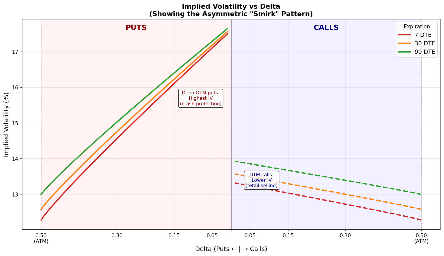
The delta vs IV chart is particularly useful since it shows the relationship in the same terms they use when selecting strikes (0.15 delta, 0.10 delta, etc.) rather than requiring us to mentally convert from moneyness.

Summary

The claim that “lower delta means lower expected value” is an artifact of assuming lognormal returns and a flat volatility surface. In reality, markets recognize fat tails and price them via skew and smile; implied volatility is typically higher on the wings, and the volatility risk premium is strike-dependent. Empirically, expected option returns are non-monotonic in moneyness — some low-delta wings are overpriced, some underpriced — so you cannot read expected value from delta alone.

The rise of retail options trading has introduced structural changes that appear to have flattened parts of the volatility surface, particularly at popular strikes. This compression of the volatility risk premium doesn’t eliminate opportunities for options sellers, but it does mean that strategies which worked well historically may need recalibration.

For protection and hedging, the implications are nuanced. Crash convexity strategies that buy deep OTM protection may actually benefit from retail-driven premium suppression on the wings, but their effectiveness still depends on execution realities during stress that are difficult to model. The safest conclusion is that any options strategy should be evaluated on its full risk-return profile, not on simplified heuristics about delta and probability.

---

Remember: Alpha is never guaranteed. And the backtest is a liar until proven otherwise.

Options and derivatives are complex instruments and not suitable for all investors. This analysis probably contains errors — if you find them, let me know.

The material presented in Math & Markets is for informational purposes only. It does not constitute investment or financial advice.

---