
CUSUM, Bayes, and the Art of Knowing When to Quit
Part 81 — Decay Series 2 of 3 — CUSUM tests, rolling Sharpe, Bayesian changepoint detection, and building a dashboard that tells you when your strategy is dying

This is part 81 of my series — Building & Scaling Algorithmic Trading Strategies
The Hardest Question in Quant Trading
You deploy a strategy and it makes money for a few months. Then it draws down for three weeks, where you lose a lot more than you made. It’s not just that you lose money but also that you don’t see it coming.
Is it a drawdown — the normal cost of doing business — or is the strategy broken?
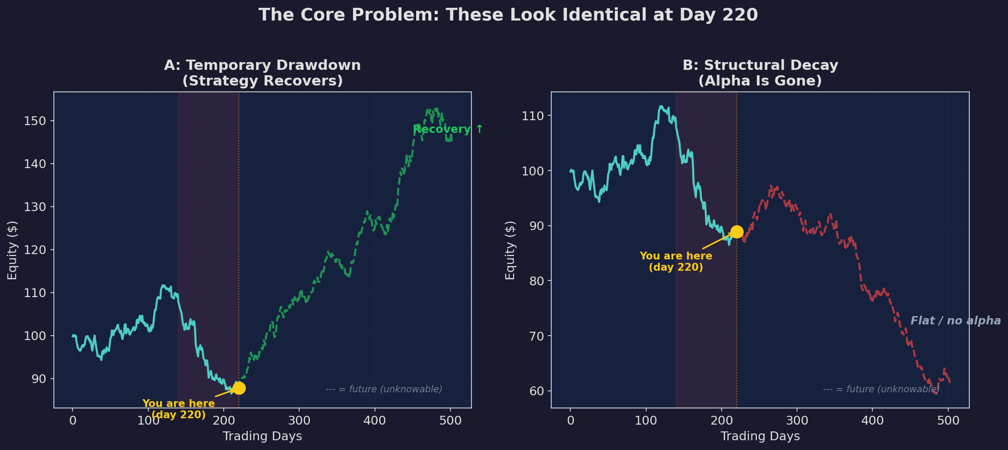
The solid blue line is identical in both panels. At day 220, you see the same equity curve, the same drawdown, the same P&L. But the future diverges completely. Scenario A recovers. Scenario B flatlines. You’re standing at the yellow dot. Which scenario are you in?
This is the fundamental problem in strategy monitoring. Drawdowns and structural decay are indistinguishable by eye during the early stages. By the time the difference is obvious, you’ve already lost months of returns.
In Part 1, I covered why strategies decay — crowding, regime change, and overfitting. This post is about detecting it before the damage is done.
The Toolkit: Four Tests, Different Trade-offs
There’s no single test that solves this problem perfectly. Every approach trades off detection speed against false alarm rate. Here’s the lineup:
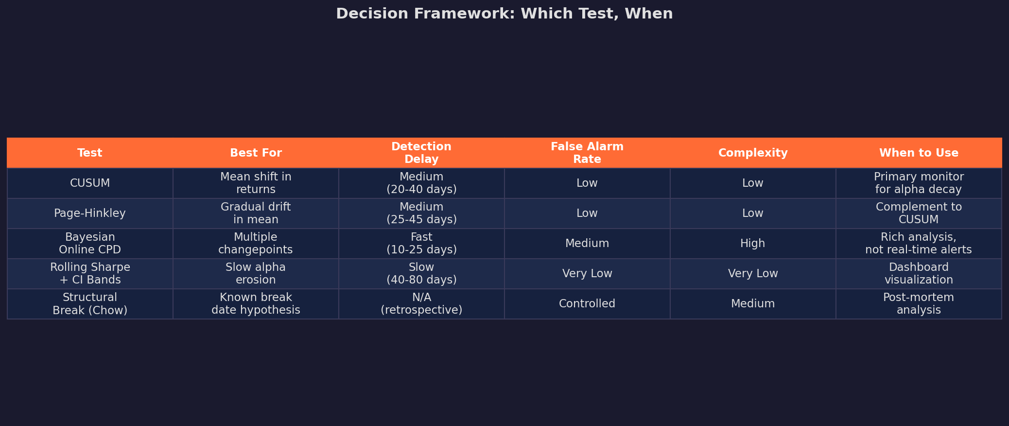
I’ll walk through each one with worked examples, starting with the most practical.
Test 1: CUSUM (Cumulative Sum Control Chart)
CUSUM is the workhorse. It was invented by E.S. Page in 1954 for industrial quality control — detecting when a manufacturing process has shifted — and it translates directly to strategy monitoring.
The idea: accumulate evidence that the process has shifted away from its expected value. Small daily deviations accumulate into a large statistic if the shift is real, but random noise resets back toward zero.
The Math
Define the one-sided CUSUM statistic for detecting a negative shift in alpha:
S⁺ₜ = max(0, S⁺ₜ₋₁ + (μ₀ - xₜ) - k)Where:
μ₀ is the expected daily return under H₀ (”strategy is working”)
xₜ is the observed daily return
k is the “allowance” or slack parameter (typically 0.5σ)
S⁺₀ = 0
When the strategy is working, daily returns are close to μ₀, so (μ₀ - xₜ) fluctuates around zero, and the max(0, ...) keeps the statistic near zero. When the strategy decays, returns fall below μ₀, the difference accumulates, and S⁺ drifts upward.
You signal an alarm when S⁺ₜ exceeds a threshold h (typically 4–5σ).
CUSUM in Action
Here’s a simulated strategy with a true changepoint at day 200 — alpha drops from ~15% annualized to approximately -5%:
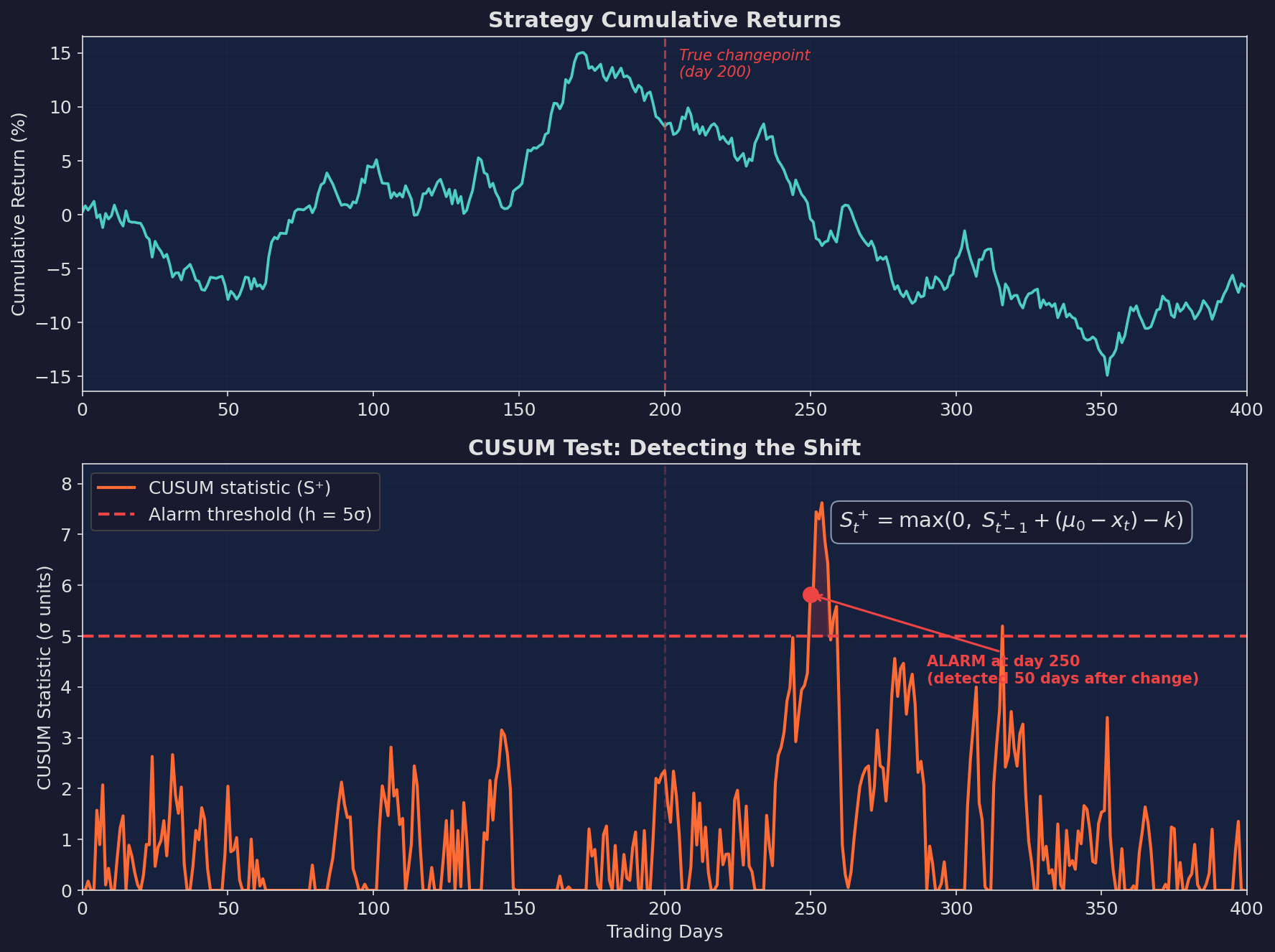
Top: cumulative returns. The curve slopes upward before day 200, then flattens and declines. Bottom: the CUSUM statistic. It stays near zero while the strategy is healthy, then climbs after the changepoint and triggers an alarm at day 250 — 50 trading days after the true change.
Fifty days of detection delay. Is that good? For a strategy running with a Sharpe of ~1, that’s about 2 months of potentially degraded returns. Not instant, but far better than waiting 6+ months for a rolling Sharpe to clearly trend negative.
Tuning the Parameters
The two knobs are k (allowance) and h (threshold):
k controls sensitivity:
  k = 0       → detects any shift, many false alarms
  k = 0.5σ    → standard setting (recommended)
  k = 1.0σ    → only detects large shifts

h controls the trade-off:
  h = 3σ      → fast detection, ~1-2 false alarms per year
  h = 4σ      → balanced (~0.5 false alarms per year)
  h = 5σ      → slow detection, very few false alarms
For strategy monitoring, I’d start with k = 0.5σ and h = 4σ. You can calibrate from there based on your tolerance for false alarms versus detection delay.
The Key Limitation
CUSUM requires you to specify μ₀ — the “expected” return under normal conditions. This is harder than it sounds. If you use the full backtest mean, you’re including the regime you’re trying to detect. If you use a short calibration window, you’re sensitive to the choice of window.
My approach: use the mean return from a clean, out-of-sample validation period. For V6, that’s the walkforward validation period we discussed in Part 32.
Test 2: Page-Hinkley Test
Page-Hinkley is CUSUM’s cousin. Well, second cousin maybe. Instead of resetting to zero, it tracks the cumulative deviation from the running mean:
mₜ = (1/t) · Σᵢ xᵢ                    (running mean)
Uₜ = Σᵢ (xᵢ - mₜ - δ)                 (cumulative deviation)
PHₜ = Uₜ - min(U₁, U₂, ..., Uₜ)       (test statistic)
Where δ is a tolerance parameter (similar to k in CUSUM).
Alarm when PHₜ > λ (the threshold).
The practical difference from CUSUM: Page-Hinkley adapts its reference point over time (via the running mean), which makes it better at detecting gradual drift versus sudden shifts. CUSUM is better for clean breaks; Page-Hinkley handles slow erosion.
For strategy monitoring, I run both in parallel — CUSUM for sudden breakdowns (regime changes) and Page-Hinkley for slow decay (crowding, signal erosion).
Test 3: Rolling Sharpe with Confidence Bands
This is the least sophisticated but most intuitive approach. Calculate the Sharpe ratio over a rolling window and watch for it to trend toward zero.
Adding Statistical Rigor
The raw rolling Sharpe is noisy. A 63-day window produces Sharpe estimates with a standard error of approximately:
SE(SR) ≈ √((1 + 0.5·SR²) / n)For a true Sharpe of 1.0 and n = 63 days:
SE ≈ √((1 + 0.5) / 63) ≈ 0.154Annualized, that’s SE × √252 ≈ 2.45. Your 95% confidence interval around a “true” annualized Sharpe of 1.0 is roughly (-3.9, 5.9).
This is absurdly wide. Which is the core problem with rolling Sharpe: by the time you have enough data to be statistically confident the Sharpe has changed, you’ve already lost a lot of money.
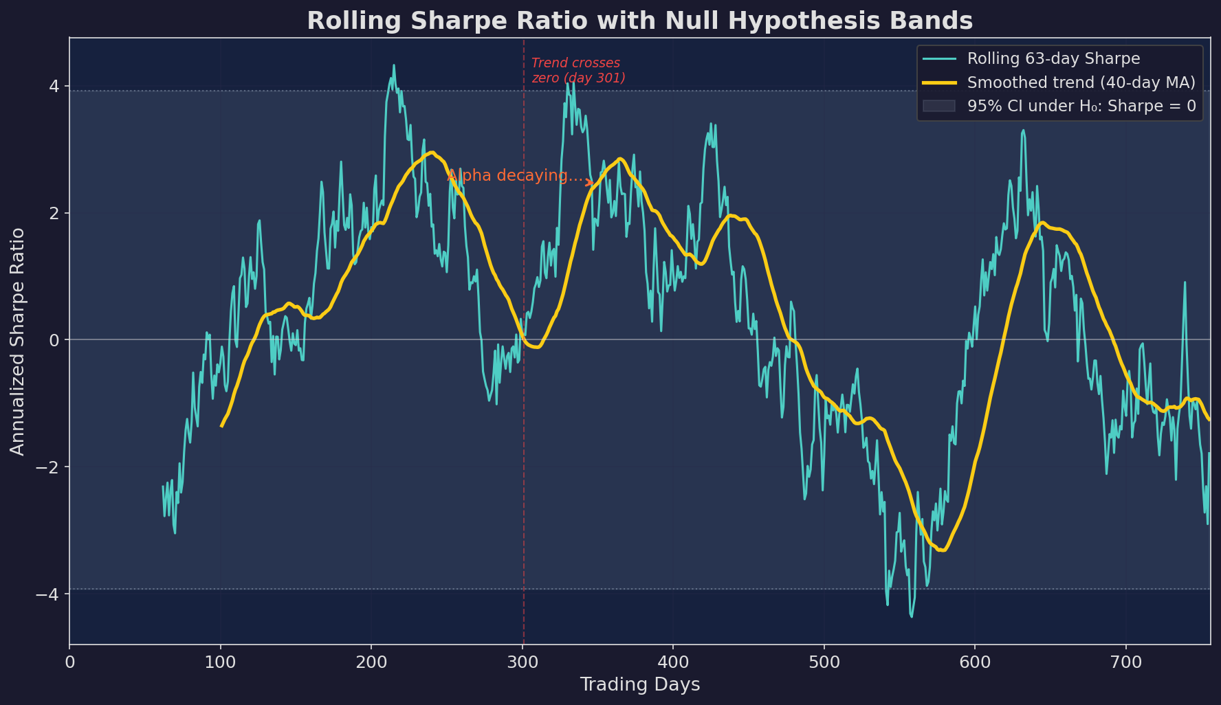
Blue: raw 63-day rolling Sharpe. Yellow: smoothed trend. Gray band: 95% confidence interval under the null hypothesis (Sharpe = 0). The rolling Sharpe can wander well outside the null band while alpha is positive, then gradually drift back toward zero as the strategy decays.
When Rolling Sharpe Is Useful
Despite the wide confidence intervals, rolling Sharpe is good for two things:
Trend detection. Apply a moving average to the rolling Sharpe. If the smoothed trend is declining over 3-6 months, that’s a signal — even if the point estimate hasn’t crossed zero yet.
Dashboard visualization. It’s the easiest metric for a quick glance. Is the Sharpe trending up, flat, or down? You don’t need to explain CUSUM to a non-quant collaborator, but everyone understands “the risk-adjusted returns are declining.”
Test 4: Bayesian Online Changepoint Detection
This is the most powerful and most complex approach. Instead of testing “has a change occurred?” (binary), it estimates “what is the probability that a change occurred at each point in time?” (continuous).
The Framework
The Bayesian approach maintains a probability distribution over the “run length” — how long since the last changepoint. At each new observation, it updates two things:
The growth probability: the data is consistent with the current regime continuing.
The changepoint probability: the data suggests a new regime has started.
P(rₜ = 0 | x₁:ₜ) ∝ Σᵣ P(xₜ | rₜ₋₁) · P(rₜ₋₁ | x₁:ₜ₋₁) · H(rₜ₋₁)Where H(r) is the hazard function — the prior probability of a changepoint at any given time.
In practice, you’re running a recursive Bayesian filter that maintains a distribution over “how long has the current regime been running?” and updates it with each new return observation.
What It Looks Like
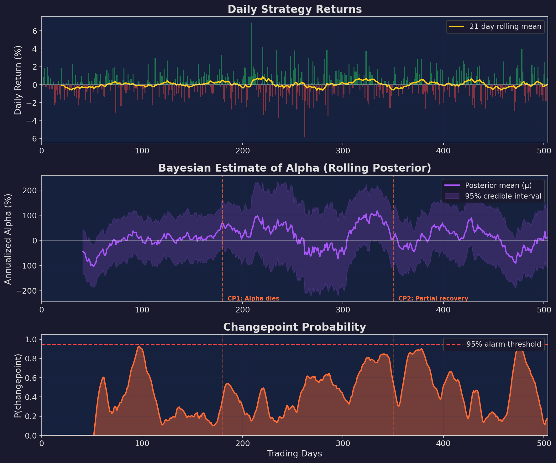
Top: daily returns with a rolling mean. Middle: Bayesian posterior estimate of annualized alpha with 95% credible interval. The interval shrinks as evidence accumulates, then widens around changepoints. Bottom: estimated probability that a changepoint has occurred. Spikes above the 95% threshold indicate detected regime changes.
Why Bayesian Is Better (and Worse)
Better: it gives you probabilities, not binary alarms. “There’s a 73% chance alpha shifted negative last week” is more useful than “ALARM” or “NO ALARM.”
Better: it naturally handles multiple changepoints. CUSUM needs to be reset after an alarm. The Bayesian filter adapts continuously.
Worse: it’s computationally heavier and requires specifying prior distributions. The choice of hazard function (how often do you expect changepoints?) and the likelihood model (are returns normally distributed?) affect results significantly.
Worse: it can be harder to calibrate. With CUSUM, you have two knobs (k, h). With Bayesian CPD, you have a prior over run lengths, a likelihood model, and hyperparameters for both.
For V6 monitoring, I’d implement Bayesian CPD for weekly analysis and retrospective study, while running CUSUM for real-time alerts.
The Fundamental Trade-off
Every test lives on the same curve: faster detection means more false alarms. Slower detection means larger losses before you act.
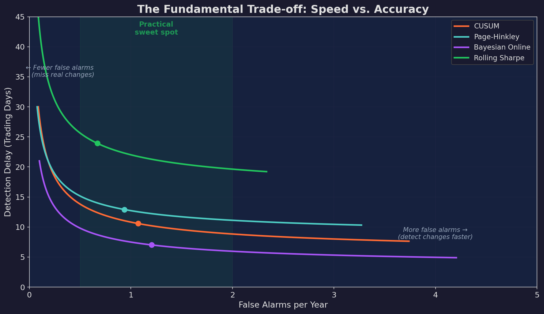
Each test traces a curve in detection-delay / false-alarm space. The “sweet spot” for most strategies is 0.5–2 false alarms per year with 20–40 days of detection delay.
The practical implication: don’t rely on a single test. Stack them.
Alert Level    Trigger                              Action
──────────────────────────────────────────────────────────────
GREEN          All tests normal                     Continue trading
YELLOW         Rolling Sharpe trend declining OR     Reduce position size 50%
               CUSUM > 70% of threshold
ORANGE         CUSUM alarm fired OR                  Halt new trades,
               Bayesian P(change) > 80%              review fundamentals
RED            Multiple tests alarming,              Full stop. Paper trade
               confirmed by Bayesian analysis        until edge reconfirmed
Building the Dashboard
Here’s what a monitoring dashboard looks like in practice, applied to simulated V6 returns:
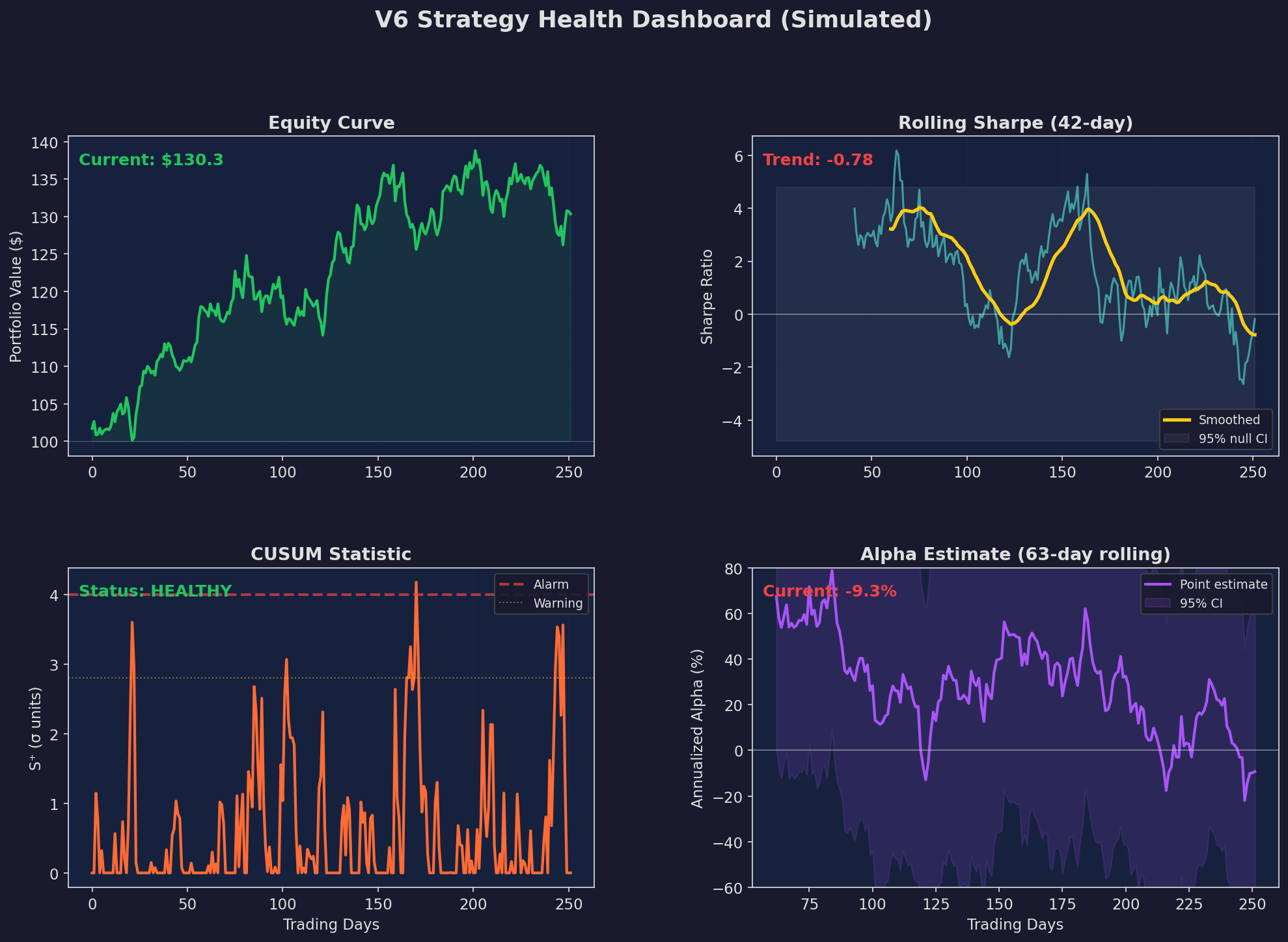
Four panels showing the key metrics at a glance. The equity curve provides context. Rolling Sharpe shows the trend. CUSUM gives the formal alarm status. The alpha posterior shows the current best estimate with uncertainty.
This dashboard takes maybe 50 lines of Python to build with matplotlib and runs in under a second. No fancy infrastructure needed. I update it daily as part of the morning trading workflow.
The key design principle: every panel answers a different question.
The equity curve answers: “am I making money?” The rolling Sharpe answers: “is my risk-adjusted performance trending?” The CUSUM answers: “has something structurally changed?” The alpha posterior answers: “what’s my best estimate of current edge, with uncertainty?”
The Real-World Complications
Everything above assumes stationary noise and clean changepoints. Reality is messier:
Non-normal returns. Strategy returns have fat tails, which inflate both the CUSUM statistic and the Sharpe estimate. Use robust estimators (median, MAD) or fit a Student-t likelihood in the Bayesian framework.
Multiple strategies. If you’re monitoring five strategies simultaneously, you’ll get a false alarm from at least one of them every few months. Apply a Bonferroni or FDR correction: if monitoring N strategies, use a threshold of h + σ·√(2·ln(N)).
Correlated returns. If your strategy is correlated with the market, a broad drawdown can trigger false alarms. Monitor alpha (returns minus benchmark) rather than raw returns.
Survivorship in your own analysis. You’ll naturally pay more attention to tests that alarm at convenient times. Be honest with yourself about how you’d act on each alert level before the alarm fires.
Implications for V6
I’m considering the following as a concrete plan for V6:
Daily. Run CUSUM with k = 0.5σ, h = 4σ on V6’s excess returns (over SPY). Auto-email if CUSUM crosses 70% of threshold.
Weekly. Update rolling 42-day and 63-day Sharpe ratios. Compare to the null bands. Run Page-Hinkley in parallel.
Monthly. Full Bayesian changepoint analysis on the trailing 6 months. Estimate posterior probability of alpha shift. Review whether the fundamental assumptions (negative stock/bond correlation, momentum persistence) still hold.
Quarterly. Structural break test (Chow test) against the most recent quarter to compare with the validation period from Part 32. Comprehensive review.
Up Next
Part 3: Adaptive Strategies — If decay is inevitable, can a strategy evolve to stay ahead of it? We’ll look at parameter drift, online learning, and the tension between adaptation and overfitting. Spoiler: this is harder than it sounds.
Remember: Alpha is never guaranteed. And the backtest is a liar until proven otherwise.
These posts are about methodology, not recommendations. If you find errors in my math, let me know — I’ve built an entire series around discovering my own mistakes, so one more won’t hurt.
The material presented in Math & Markets is for informational purposes only. It does not constitute investment or financial advice.