
Can a Strategy Evolve? The Math of Adaptation vs. Overfitting
Part 82 — Decay Series 3 of 3 — Online learning, walkforward optimization, forgetting factors, and why the obvious answer is wrong

This is part 82 of my series — Building & Scaling Algorithmic Trading Strategies
The Obvious Solution That Isn’t
In Part 1, we discussed how almost all strategies decay — momentum signals with a half-life of 18-24 months, VIX signals with 12-18 months, short-term reversal with just 6-12 months. In Part 2, we talked through building a detection toolkit: CUSUM, Bayesian changepoint detection, rolling Sharpe with null bands.
So the natural next question for us is if the optimal parameters drift over time, why not just... update them?
Refit the model. Roll the window. Use online learning. Let the strategy adapt. Sounds pretty cool right?
I mean, it sounds so obvious but realistically it’s also a trap. The same mechanism that allows a strategy to adapt to changing markets also allows it to overfit to noise in real-time. And overfitting isn’t obvious at first, because we all like to think it’s just our great instincts, which is what makes it really hard.
Besides, adaptation and overfitting are the same mathematical operation — the difference is whether you’re tracking a real shift or chasing randomness.
This post is about finding the line between them.
The Adaptation Spectrum
There’s a continuum of approaches, from fully static to fully adaptive:
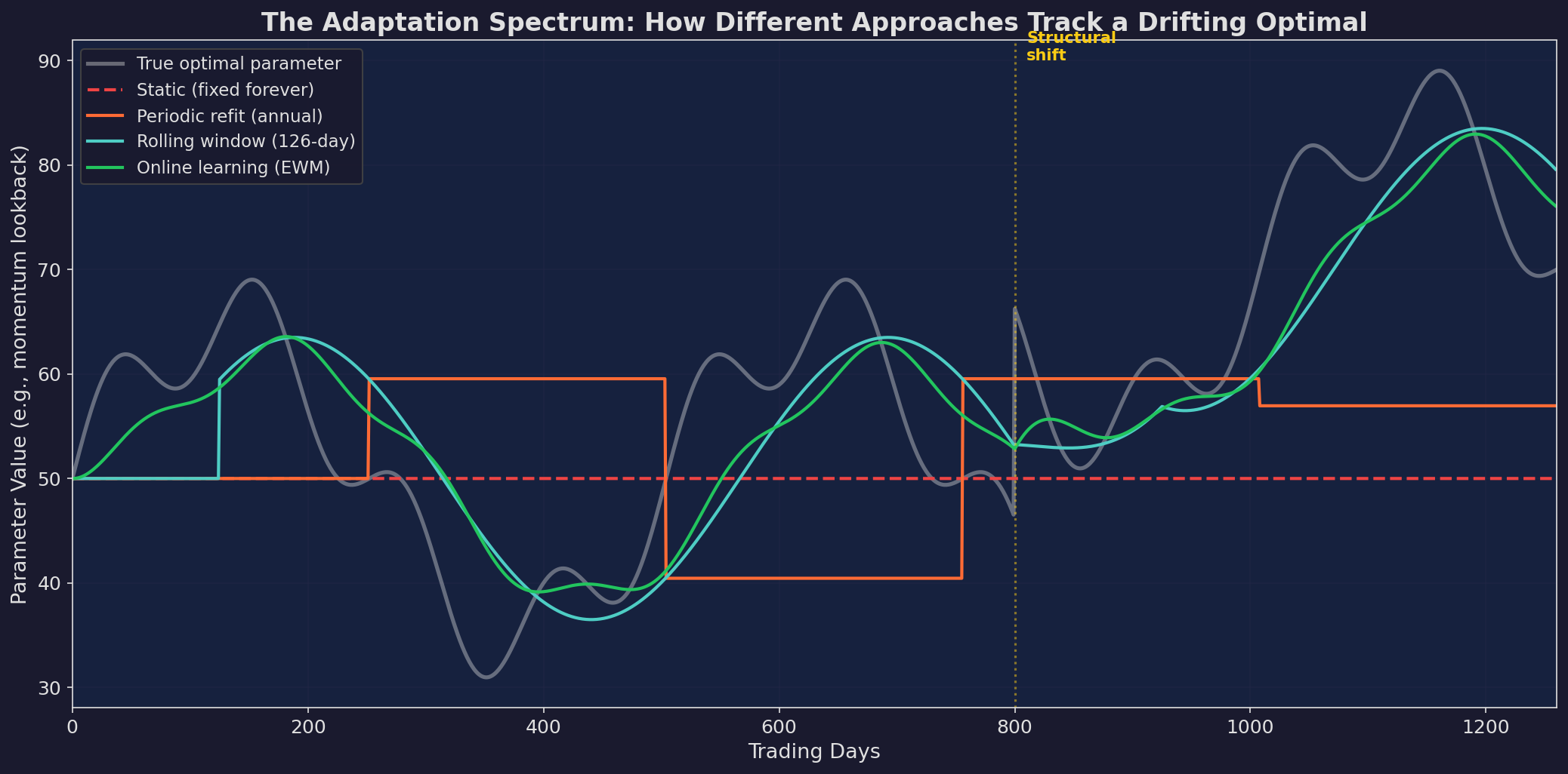
White line: the “true” optimal parameter drifting over time. Red dashed: static strategy that never updates (increasingly wrong). Orange steps: periodic annual refit (catches broad trends, misses details). Blue: 126-day rolling window. Green: exponentially weighted online learning. Each approach trades off responsiveness against stability.
Five approaches, ranked by adaptiveness:
Approach           Responsiveness    Overfit Risk    Complexity
──────────────────────────────────────────────────────────────
Static             None              None            Zero
Periodic refit     Low               Low             Low
Rolling window     Medium            Medium          Low
Online learning    High              High            Medium
Full ML retraining Very high         Very high       High
The key insight from the chart: no approach tracks the true optimal perfectly. The rolling window (blue) and online learning (green) are closest, but they also oscillate more — tracking noise, not just signal.
After the structural shift at day 800, the static strategy is permanently wrong. The periodic refit catches it a year late. The rolling window and online learner adjust within 2-3 months. But that speed comes with a cost visible in the rest of the chart: they also “adapt” to random fluctuations that mean nothing.
The Bias-Variance Trade-off (Again)
If you’ve taken an ML course, you’ve seen this. But it applies differently in finance because the data is non-stationary.
In classical statistics, the bias-variance trade-off is about model complexity: too simple = high bias (underfitting), too complex = high variance (overfitting).
In strategy adaptation, the trade-off is about window length:
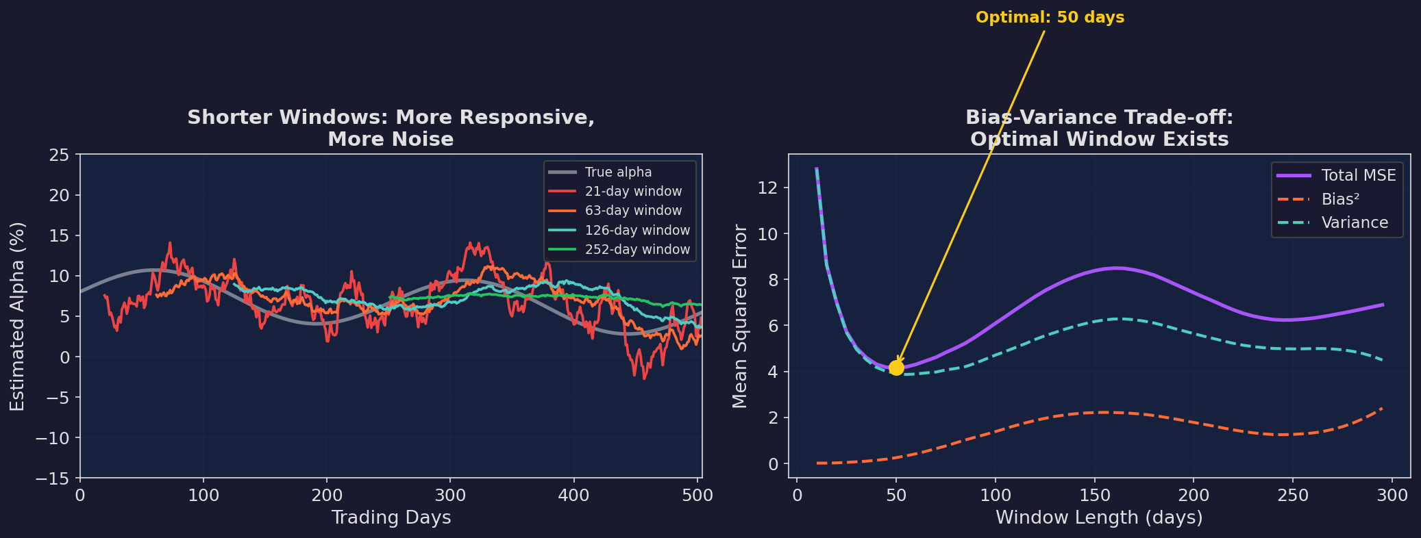
Left: shorter windows are more responsive but noisier. The 21-day estimate (red) oscillates wildly. The 252-day estimate (green) is smooth but systematically wrong — it can’t track the declining trend. Right: the mean squared error has a minimum around 60-80 days. Shorter than that, you’re overfitting to noise. Longer, you’re missing real drift.
The math is clean. For a parameter μ that drifts at rate δ per day, estimated using a rolling window of length w:
Bias²    = (δ · w / 2)²          ← grows with window length
Variance = σ² / w                 ← shrinks with window length
MSE      = Bias² + Variance
         = (δw/2)² + σ²/w
Taking the derivative and setting to zero:
dMSE/dw = δ²w/2 - σ²/w² = 0
w* = (2σ² / δ²)^(1/3)
For a strategy with daily return noise σ = 1% and parameter drift δ = 0.01% per day:
w* = (2 × 0.01² / 0.0001²)^(1/3)
   = (2,000,000)^(1/3)
   ≈ 126 days
Approximately 6 months. Which is suspiciously close to the “quarterly refit” heuristic that many quant shops use. Sometimes the rules of thumb are right.
The Goldilocks Problem: How Often Should You Refit?
Theory says ~126 days. But that assumes you know the drift rate δ, which you don’t. And it assumes the drift is constant, which it isn’t.
I simulated this across 200 Monte Carlo paths with drifting parameters:
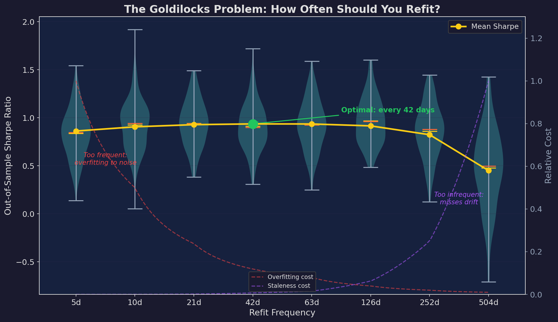
Violin plots show the distribution of out-of-sample Sharpe ratios across simulations. The mean (yellow line) peaks around 42 days. The dashed curves decompose the error: overfitting cost (red) decreases with longer windows while staleness cost (purple) increases. The crossing point defines the optimum.
The takeaways:
Too frequent (5-10 days): The mean Sharpe is lower and the variance is higher. You’re getting whipsawed. The parameter estimate is dominated by the last week of noise.
Too infrequent (252-504 days): Lower mean Sharpe because you’re systematically stale. You miss regime changes by 6-12 months.
The sweet spot (21-63 days): Highest mean Sharpe with acceptable variance. Monthly to quarterly refitting balances responsiveness against noise.
One detail that matters: the variance is widest on the left side of the chart. High-frequency refitting doesn’t just give you worse average performance — it gives you more unpredictable performance. You might get lucky with a 5-day refit window, but you’re more likely to get unlucky.
Walkforward Optimization: The Right Way to Refit
If you’re going to refit, the methodology matters enormously. The wrong way: re-optimize on the full historical dataset every time. That’s just expanding-window overfitting.
The right way: walkforward optimization. Train on a fixed-length window, test on the next period, slide forward, repeat.
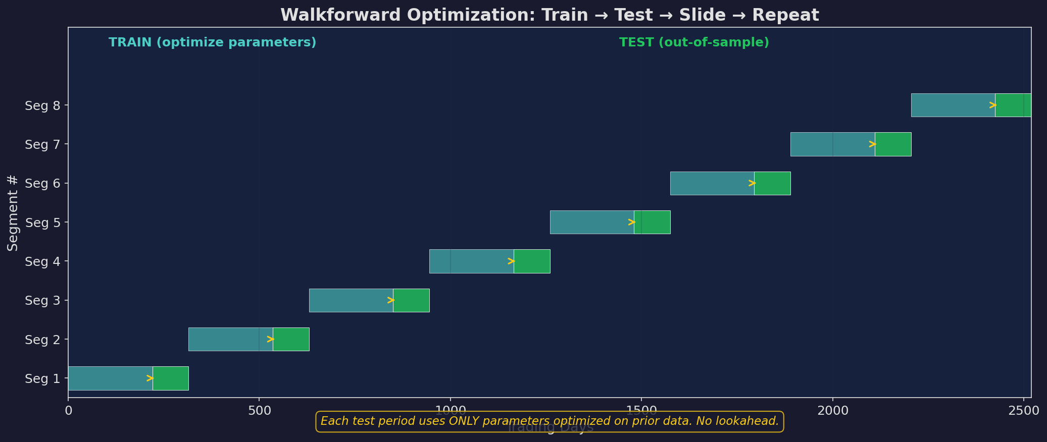
Each segment uses only prior data for optimization and tests on future data. The test periods, stitched together, form a continuous out-of-sample equity curve.
The rules are as follows…
1. Training window ≥ 2× test window. If you test on 63 days, train on at least 126 — less than that, and your parameter estimates are too noisy.
2. No peeking. The test period parameters are locked before you see test period data. Any modification during the test period invalidates the out-of-sample claim.
3. Stitch the test periods. Your “real” equity curve is the concatenation of all test periods. This is the only performance number that matters.
4. Track parameter stability across segments. If the optimal momentum threshold is 0.1% in segment 1, 0.3% in segment 2, 0.05% in segment 3, and 0.4% in segment 4, you don’t have a stable signal — you have noise.
For V6, the walkforward structure I use:
Training:  126 trading days (~6 months)
Testing:    63 trading days (~3 months)
Slide:      63 days (non-overlapping test periods)
Parameters: momentum threshold, VIX boundaries
Forgetting Factors: How Fast Should the Strategy Learn?
An alternative to discrete refitting is continuous learning via exponential weighting. Instead of a hard window, old data fades gradually:
μ̂ₜ = (1 - λ) · μ̂ₜ₋₁ + λ · xₜWhere λ is the “learning rate” or “forgetting factor.” Higher λ = faster adaptation.
The effective window length is approximately 1/λ. So λ = 0.02 corresponds to roughly a 50-day window, and λ = 0.005 corresponds to roughly 200 days.
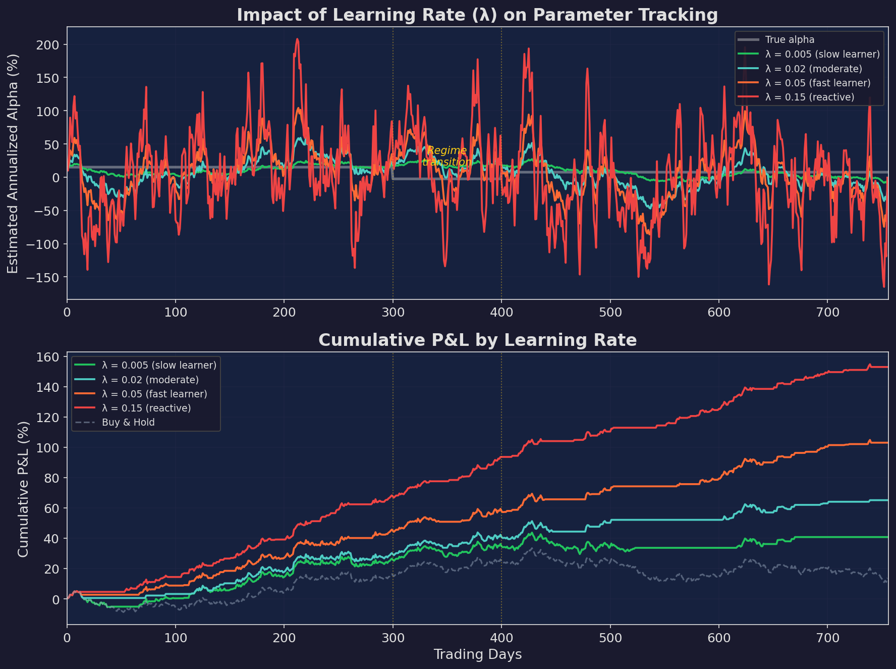
Top: how different learning rates track the true alpha. The slow learner (green, λ=0.005) barely notices the regime change. The fast learner (red, λ=0.15) oscillates wildly in both regimes. The moderate learner (blue, λ=0.02) finds the balance. Bottom: cumulative P&L when using each estimate to make allocation decisions.
The regime change happens around day 300-400: alpha drops from ~15% to ~7.5% annualized. Watch how each learning rate handles it:
Slow (λ = 0.005): Still thinks alpha is 15% at day 500. Overallocated for 200+ days.
Fast (λ = 0.15): Detects the shift quickly, but oscillates so much that its allocation decisions are essentially random. The P&L shows the damage: constant whipsaw.
Moderate (λ = 0.02): Adjusts within ~60 days. Not perfect, but the P&L shows the benefit: it captures most of the upside in the first regime and limits damage in the transition.
Choosing λ
The optimal λ depends on the same parameters as the optimal window length:
λ* ≈ √(δ² / (2σ²))For σ = 1% daily noise and δ = 0.01% daily drift:
λ* ≈ √(0.0001² / (2 × 0.01²)) ≈ 0.007This corresponds to an effective window of ~140 days. Consistent with the walkforward analysis.
In practice, I’d recommend starting with λ = 0.01 (effective 100-day window) and adjusting based on your CUSUM monitoring from Part 2. If CUSUM is alarming frequently, your λ is too low (you’re adapting too slowly). If your P&L shows whipsaw, your λ is too high.
The Adaptation Paradox
Here’s the punchline of this series: moderate adaptation beats both extremes.
I simulated three approaches over 10 years of synthetic data with regime changes:
Green (moderate adaptation) wins on both Sharpe ratio and max drawdown. Static (gray) takes the full force of every bear market. Hyper-adaptive (red) gets whipsawed during choppy periods, missing recoveries while sitting in cash.
The numbers tell the story clearly:
The static approach takes every drawdown on the chin — 74% max drawdown over 10 years. It ends slightly positive but the ride is brutal.
The hyper-adaptive approach tries to dodge drawdowns by switching to cash whenever the 21-day Sharpe turns negative. The problem: it also switches to cash during normal pullbacks within bull markets, then misses the recovery. Every chop zone becomes a series of buys near the top and sells near the bottom.
The moderate approach scales down gradually when evidence accumulates over 63 days. It doesn’t dodge every drawdown — it still takes hits. But it avoids the worst of them while maintaining enough exposure to capture recoveries.
What Not to Adapt
Not everything should be adaptive. Some components of a strategy are better left fixed:
Adapt: Position sizing, momentum threshold, allocation weights between assets.
Don’t adapt: The fundamental structure of the strategy (e.g., “momentum works”), the risk management rules (e.g., max drawdown tolerance), the instruments traded.
Why? Adapting the structure is equivalent to strategy selection, which requires an order of magnitude more data. You can estimate an optimal momentum threshold with 126 days of data. You cannot determine whether momentum still works as a concept with 126 days of data.
For V6 specifically:
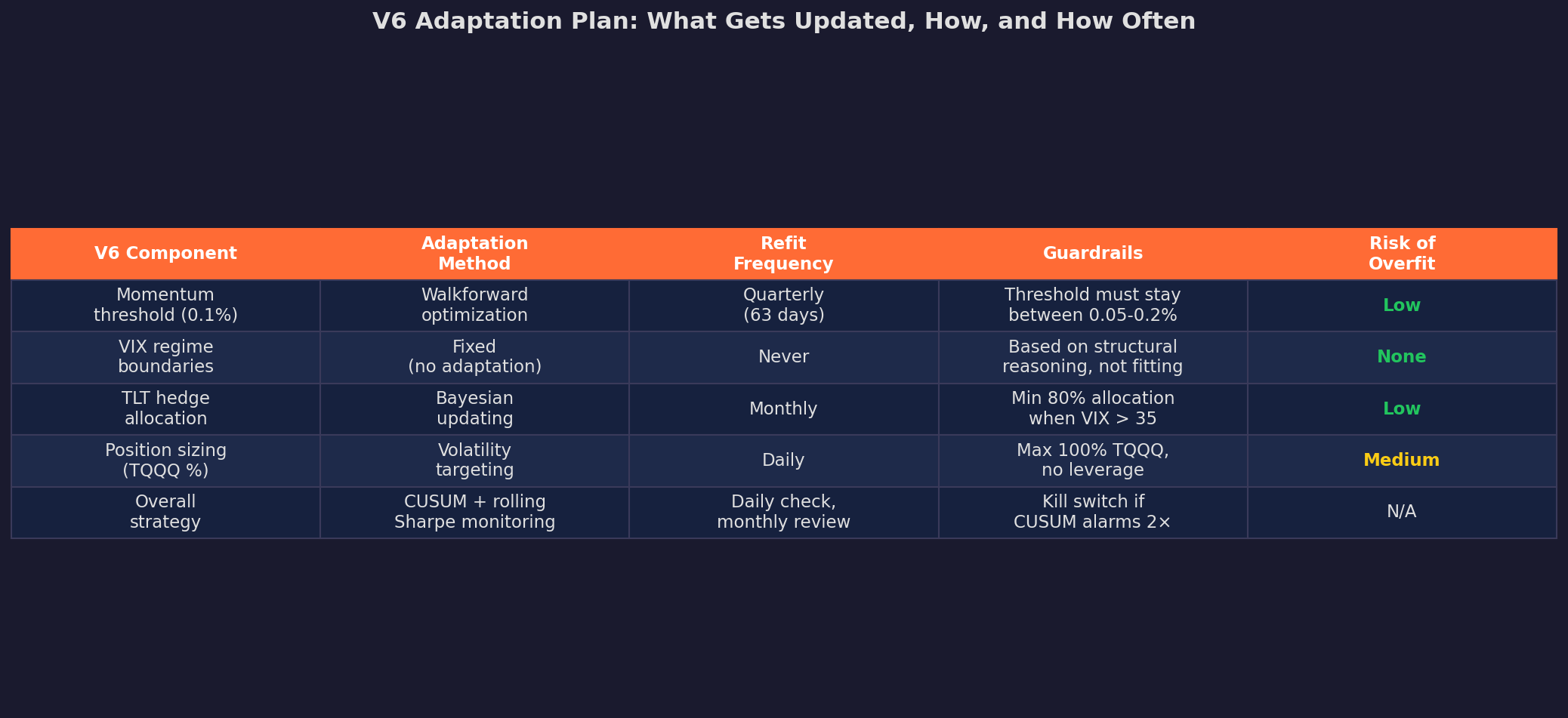
The key design choice: VIX regime boundaries are fixed and never adapted. These aren’t fitted parameters — they’re based on structural reasoning about what VIX levels correspond to different market states. Adapting them would mean the strategy is learning “when to be scared,” which is exactly the kind of thing that overfits.
Meanwhile, the momentum threshold is adapted quarterly via walkforward optimization, because the speed of trends genuinely changes over time. And position sizing uses daily volatility targeting, which is the most adaptive component — but with hard guardrails (max 100% TQQQ, no leverage).
The Hierarchy of Adaptation
If I had to distill this entire series into a single framework, it’s this:
Level 1: Monitor (always)
  → CUSUM, rolling Sharpe, Bayesian CPD
  → Cost: zero (just watching)
  → Benefit: early warning

Level 2: Scale positions (daily)
  → Volatility targeting, risk budgeting
  → Cost: some tracking error
  → Benefit: smooth equity curve

Level 3: Refit parameters (quarterly)
  → Walkforward optimization on tactical parameters
  → Cost: risk of overfitting to recent regime
  → Benefit: adapts to drift

Level 4: Review structure (annually)
  → Does the fundamental thesis still hold?
  → Cost: high (may require new strategy entirely)
  → Benefit: avoids being stuck in a dead paradigm

Level 5: Replace strategy (when evidence is overwhelming)
  → Multiple tests alarming, structural thesis broken
  → Cost: very high (starting over)
  → Benefit: survival
Most days, you’re at Level 1 and 2. Quarterly, you do Level 3. Annually, you do Level 4. Level 5 happens maybe once every 3-5 years.
The mistake most people make is oscillating between Level 0 (ignore everything) and Level 5 (blow it up and start over) with nothing in between. The whole point of this series is to fill in Levels 1-4.
What’s Next for V6
Concretely, here’s what I’m implementing based on this series:
Daily: CUSUM monitoring on excess returns (from Part 2). Volatility-targeted position sizing with 15% annualized vol target. Auto-email if CUSUM crosses 70% of alarm threshold.
Monthly: Update the EWM alpha estimate (λ = 0.01). Compare to the 63-day rolling Sharpe. If both suggest alpha < 5% annualized, scale to 50% allocation.
Quarterly: Walkforward refit of the momentum threshold. Training on prior 126 days, testing on next 63 days. Guardrails: threshold must stay between 0.05% and 0.20%.
Annually: Full structural review. Does the TLT hedge still work? Is stock/bond correlation still negative in stress? Does momentum still persist?
The system isn’t complicated but the hard part isn’t the implementation — it’s the discipline to follow it, especially when the CUSUM is flashing yellow and every instinct says to override the system.
This concludes the 3-part series on strategy decay. If you want to go deeper on any of these topics — especially the implementation details of CUSUM monitoring or walkforward optimization — let me know in the comments.
Remember: Alpha is never guaranteed. And the backtest is a liar until proven otherwise.
These posts are about methodology, not recommendations. If you find errors in my math, let me know — I’ve built an entire series around discovering my own mistakes, so one more won’t hurt.
The material presented in Math & Markets is for informational purposes only. It does not constitute investment or financial advice.