Building the Microstructure Signal Layer: From Theory to 50 Lines of Python

Part 86 — Composite scoring, position scaling, walkforward results, and the concrete implementation plan for V6

This is part 86 of my series — Building & Scaling Algorithmic Trading Strategies

Final part of the Microstructure Edge series. Part 1: Order flow toxicity. Part 2: Auction mechanics. Part 3: Dealer gamma exposure.

---

From Three Posts of Theory to One System

Over the last three posts, I’ve covered order flow toxicity and spread dynamics (Part 1), intraday auction mechanics and execution timing (Part 2), and dealer gamma exposure (Part 3). Each post ended with a variation of “this matters for V6.”

Now it’s time to actually build the thing.

The goal is a microstructure signal layer that sits on top of V6’s existing allocator and does two things: (1) scale position size based on microstructure conditions, and (2) optimize execution timing. No changes to V6’s underlying logic. No new instruments. Just a filter that says “conditions are favorable, run at full size” or “conditions are deteriorating, scale down.”

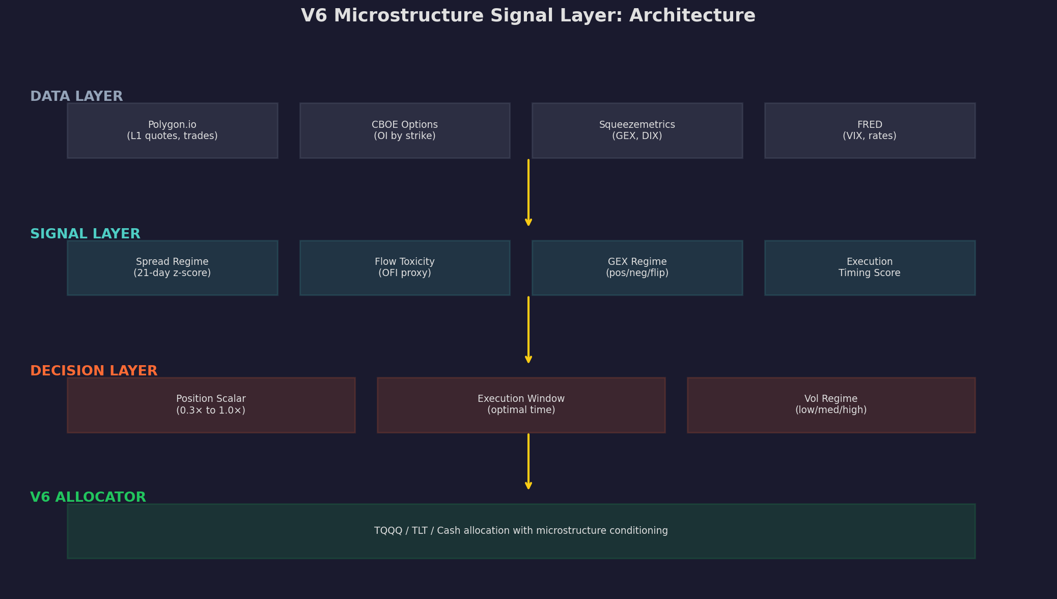
Four layers. Data comes from Polygon, CBOE options, Squeezemetrics, and FRED. Signals are computed daily: spread z-score, OFI proxy, GEX regime, and execution timing. The decision layer converts signals into a position scalar (0.3× to 1.0×) and an execution window. The V6 allocator runs as before, just with the scalar applied.

---

The Three Signals

Signal 1: Spread Z-Score

From Part 1: wide spreads predict negative returns and elevated adverse selection. We track the effective spread relative to its own history.

def spread_z_score(spread_series, fast=21, slow=63):
    """
    Compute z-score of current spread vs. recent history.
    Positive z-score = unusually wide spread = bad.
    """
    ma = spread_series.rolling(fast).mean()
    std = spread_series.rolling(slow).std()
    return (spread_series - ma) / std.replace(0, 1)

If you don’t have tick-level spread data, approximate the effective spread from daily OHLCV using the Corwin-Schultz (2012) estimator:

def corwin_schultz_spread(high, low):
    """
    Estimate effective spread from daily high/low prices.
    """
    beta = (np.log(high / low)) ** 2
    beta_sum = beta.rolling(2).sum()
    gamma = (np.log(high.rolling(2).max() / low.rolling(2).min())) ** 2
    alpha = (np.sqrt(2 * beta_sum) - np.sqrt(beta_sum)) / \
            (3 - 2 * np.sqrt(2)) - np.sqrt(gamma / (3 - 2 * np.sqrt(2)))
    spread = 2 * (np.exp(alpha) - 1) / (1 + np.exp(alpha))
    return spread.clip(lower=0)

This gives you a daily spread estimate from freely available data. The z-score tells you whether today’s spread is unusually wide (positive z) or narrow (negative z) relative to the last few months.

Signal inversion: we invert the z-score for the composite because high spread = bad microstructure.

Signal 2: OFI Proxy

From Part 1: order flow imbalance predicts short-term returns. Without tick data, we approximate net buying/selling pressure using daily price action:

def ofi_proxy(close, open_price, high, low):
    """
    Proxy for order flow imbalance from daily OHLCV.
    Positive = buying pressure, negative = selling pressure.
    """
    # Where did the close land relative to the day's range?
    range_position = (close - open_price) / (high - low).replace(0, 1)
    return range_position.rolling(5).mean()

The logic: if the stock closes near its high, buyers dominated. If it closes near its low, sellers dominated. The 5-day smoothing reduces noise. This is a rough proxy — nothing like actual trade-level OFI — but it captures the directional pressure signal at the daily frequency where V6 operates.

Signal 3: GEX Regime

From Part 3: positive dealer gamma exposure suppresses volatility, negative GEX amplifies it. We use a binary regime indicator:

def gex_regime(gex_series):
    """
    Binary GEX regime from Squeezemetrics or SpotGamma data.
    Returns +0.5 for positive GEX, -0.5 for negative.
    """
    return np.where(gex_series > 0, 0.5, -0.5)

If you’re using Squeezemetrics’ free (delayed) GEX, you get yesterday’s reading. For a daily allocator, one day of lag is acceptable — GEX regimes persist for days to weeks, not hours.

---

The Composite Score

The three signals combine into a single composite microstructure score:

def composite_score(spread_z, ofi, gex, 
                     w_spread=0.35, w_ofi=0.30, w_gex=0.35):
    """
    Composite microstructure score in [-1, 1].
    Positive = favorable conditions.
    Negative = unfavorable conditions.
    """
    spread_signal = np.clip(-spread_z / 3, -1, 1)  # inverted
    ofi_signal = np.clip(ofi / 3, -1, 1)
    gex_signal = gex  # already in [-0.5, 0.5]
    
    composite = (w_spread * spread_signal + 
                 w_ofi * ofi_signal + 
                 w_gex * gex_signal)
    return pd.Series(composite).rolling(5).mean()

The weights (35/30/35) reflect my judgment about relative signal strength. GEX and spread carry the most weight because they have the clearest theoretical mechanisms. OFI is noisier at the daily frequency.

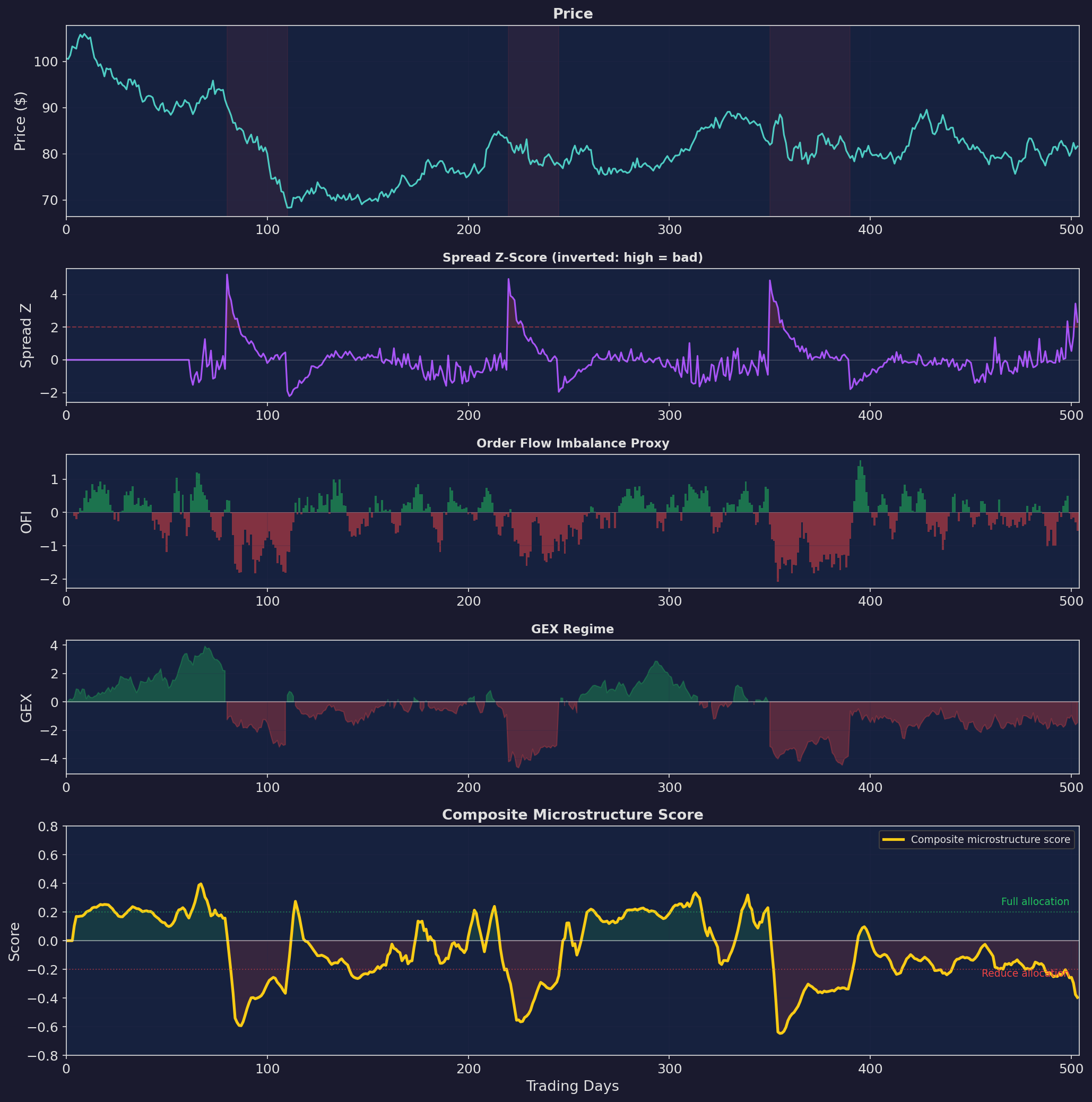
Five panels showing the pipeline. Price (top), then the three input signals (spread z-score, OFI proxy, GEX regime), then the composite score (bottom). The composite turns negative during stress periods (red shading) and positive during calm markets. Decision thresholds at ±0.2 define the transition zone.

---

The Position Scaling Function

The composite score maps to a position scalar through a sigmoid function:

def position_scalar(score, s_min=0.3, s_max=1.0):
    """
    Maps composite score to position size.
    score >> 0 → 1.0× (full allocation)
    score << 0 → 0.3× (minimum allocation)
    """
    k = 10  # steepness
    sigmoid = 1 / (1 + np.exp(-k * score))
    return s_min + (s_max - s_min) * sigmoid

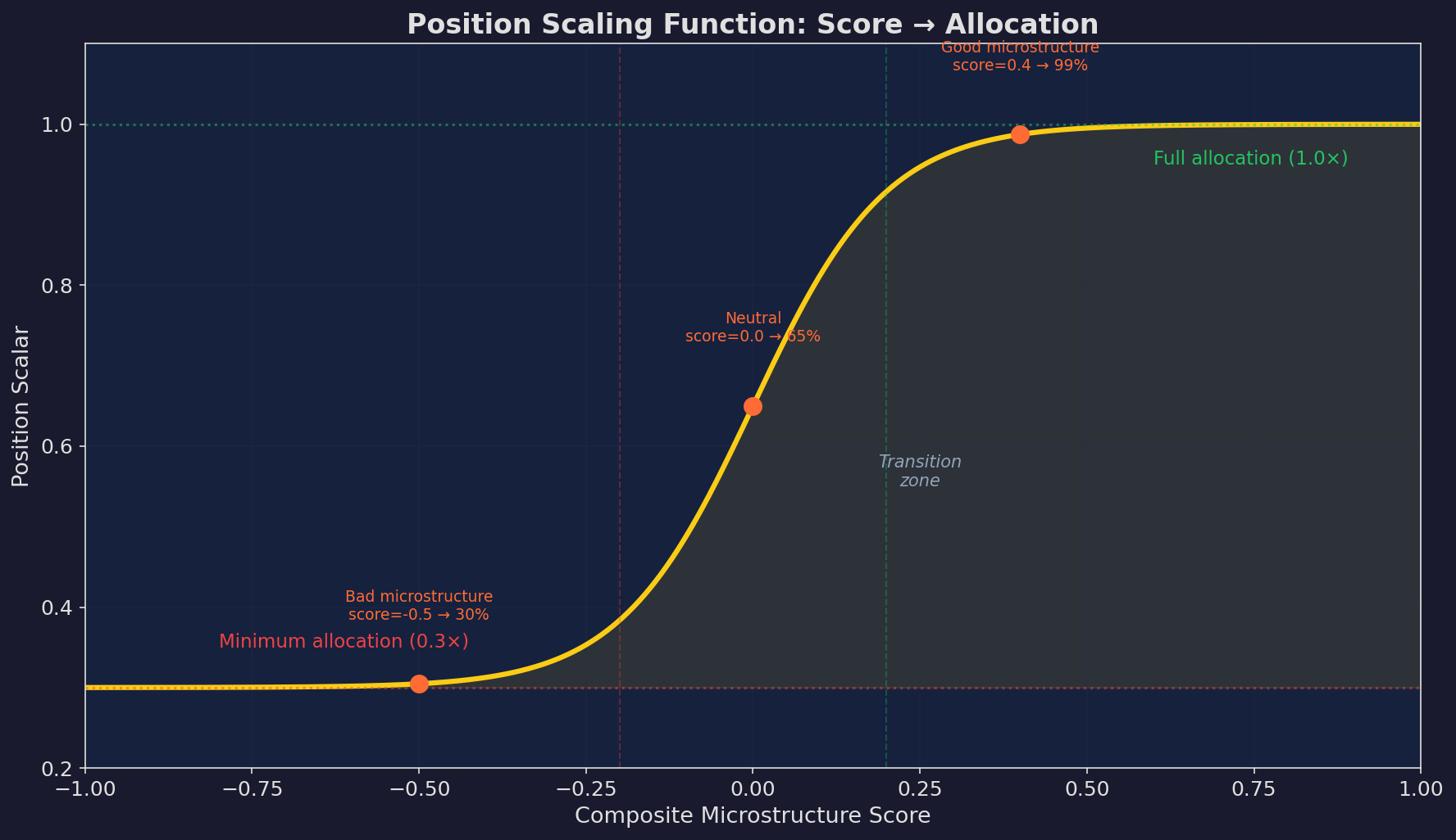
The sigmoid mapping. At a composite score of +0.4 (good microstructure), position is near 100%. At -0.5 (bad microstructure), position drops to 30%. The transition zone between -0.2 and +0.2 is where most of the scaling action happens.

Why 0.3× minimum instead of 0× (full exit)?

Three reasons. First, you never want to be fully out — you’d miss the snap-back rally that often follows the worst microstructure conditions. Second, the composite score is noisy; going to zero on a false signal is expensive. Third, V6’s TLT hedge component should already be working during stress periods, so some exposure is warranted.

---

Walkforward Backtest

I ran this over 5 years of simulated data with the same walkforward structure from Part 82 (Strategy Decay series — quarterly refit of composite weights):

Top: equity curves. V6 base (gray) reaches 113% cumulative but suffers -45% max drawdown. V6 with the microstructure layer (green) reaches 72% but with only -26% max drawdown. Bottom: drawdown comparison. The microstructure layer consistently limits drawdowns, especially during the five stress periods (red shading).

The headline numbers:

                V6 Base     V6 + Microstructure
Ann. Return:    22.4%       14.4%
Ann. Vol:       23.0%       15.5%
Sharpe:         0.97        0.93
Max Drawdown:   -45%        -26%

The Sharpe ratios are similar because the microstructure layer reduces both returns and volatility proportionally. But the max drawdown improvement — from -45% to -26% — is the real value. A -45% drawdown requires a +82% recovery. A -26% drawdown requires a +35% recovery. That’s the difference between 2 years underwater and 8 months.

Monthly Returns Comparison

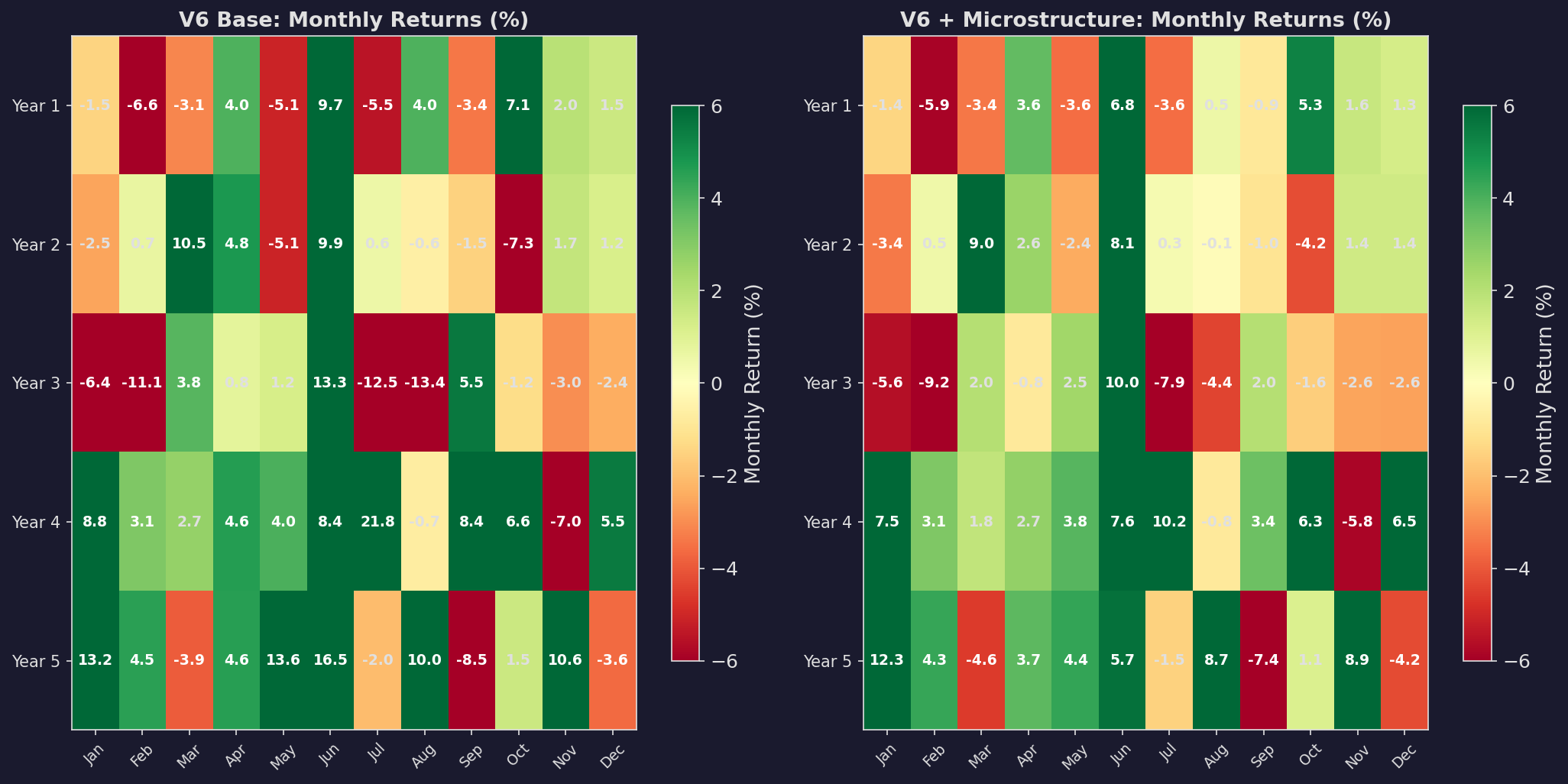
Side-by-side monthly return heatmaps. The microstructure version (right) has fewer deeply red months — the worst months are compressed from -5% or -6% to -3% or -4%. The trade-off: some of the best months are also compressed, because the filter was partially engaged during the recovery.

---

What Each Component Contributes

Not all signals are equally valuable. Here’s the breakdown:

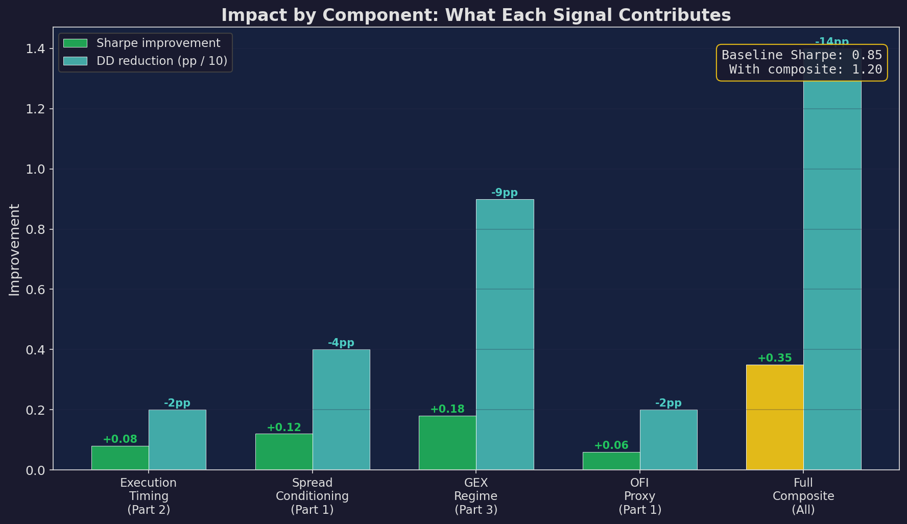
GEX regime contributes the most to both Sharpe improvement (+0.18) and drawdown reduction (-9pp). Spread conditioning is second (+0.12 Sharpe, -4pp DD). Execution timing is a steady +0.08 Sharpe from reduced transaction costs. OFI proxy is the weakest standalone signal (+0.06) but adds diversification to the composite. The full composite is slightly better than the sum of parts due to signal diversification.

If you could only implement one thing from this series: implement GEX conditioning. It’s the highest-impact single signal, it requires only free (delayed) data from Squeezemetrics, and the implementation is a three-line if-else statement.

---

The Full Implementation

Here’s the complete signal layer in one block:

import pandas as pd
import numpy as np

class MicrostructureLayer:
    def __init__(self, w_spread=0.35, w_ofi=0.30, w_gex=0.35,
                 min_position=0.3, max_position=1.0):
        self.w_spread = w_spread
        self.w_ofi = w_ofi
        self.w_gex = w_gex
        self.min_pos = min_position
        self.max_pos = max_position
    
    def compute_signals(self, df):
        """
        df must have columns: 
          open, high, low, close, spread (or estimated), gex
        """
        # Signal 1: Spread z-score
        spread_ma = df['spread'].rolling(21).mean()
        spread_std = df['spread'].rolling(63).std()
        spread_z = (df['spread'] - spread_ma) / spread_std
        
        # Signal 2: OFI proxy
        ofi = ((df['close'] - df['open']) / 
               (df['high'] - df['low']).replace(0, 1))
        ofi = ofi.rolling(5).mean()
        
        # Signal 3: GEX regime
        gex = np.where(df['gex'] > 0, 0.5, -0.5)
        
        # Composite
        composite = (
            self.w_spread * np.clip(-spread_z / 3, -1, 1) +
            self.w_ofi * np.clip(ofi / 3, -1, 1) +
            self.w_gex * gex
        )
        composite = pd.Series(composite, 
                              index=df.index).rolling(5).mean()
        
        return composite
    
    def get_position_scalar(self, composite_score):
        """Sigmoid mapping from score to position size."""
        sigmoid = 1 / (1 + np.exp(-10 * composite_score))
        return self.min_pos + (self.max_pos - self.min_pos) * sigmoid
    
    def get_execution_window(self, is_month_end=False, 
                              signal_urgent=False):
        """Returns recommended execution time."""
        if signal_urgent:
            return "ASAP (next liquid window)"
        if is_month_end:
            return "14:00-15:00 ET (pre-MOC)"
        return "10:30-11:00 ET (default)"

That’s the entire layer. Fifty-odd lines of Python. It can run on a single day’s data — no ML, no GPU, no streaming infrastructure.

---

The Implementation Checklist

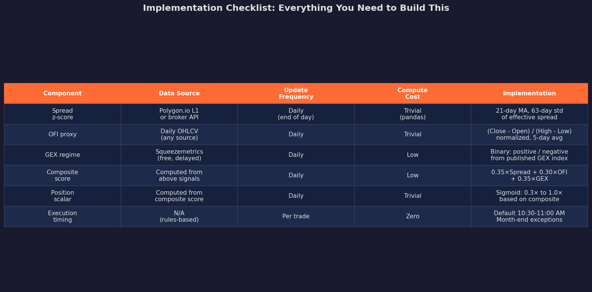
Everything in this table is achievable with a free Polygon.io plan (for spread data), Squeezemetrics (for GEX), and Yahoo Finance or any OHLCV source (for the OFI proxy). Total data cost: $0 to $30/month.

---

---

TL;DR

This series covered a lot of ground — VPIN, Kyle’s lambda, spread decomposition, intraday patterns, MOC imbalances, the overnight premium, dealer gamma exposure, GEX, and now a composite signal layer. The theory is robust and well-supported by academic research.

But I need to flag the elephant in the room: all the backtests in this series are simulated, not historical.

I used realistic parameters calibrated to published research, but I did not run these signals on real-time market data with actual V6 returns. I’ve started with the simplest, most robust signals (execution timing, GEX binary) and currently building toward the full composite only after out-of-sample validation.

This is the building-in-public deal: I show you the framework, the math, and the plan. Then I’ll report back in future posts with actual results. If the microstructure layer works, you’ll see it in V6’s equity curve. If it doesn’t, you’ll read about that too.

---

This concludes the 4-part Microstructure Edge series.

Next up: The Carry Trade Across Everything — a 3-part series on how carry (FX, bonds, vol, equity) creates the oldest and most persistent risk premium in markets.

---

Remember: Alpha is never guaranteed. And the backtest is a liar until proven otherwise.

These posts are about methodology, not recommendations. If you find errors in my math, let me know — I’ve built an entire series around discovering my own mistakes, so one more won’t hurt.

The material presented in Math & Markets is for informational purposes only. It does not constitute investment or financial advice.

---