
Adding Options to V6: Attempting to Push Dual Allocator Sharpe Above 1.0
Part 39 explores whether options can reduce drawdown and improve Sharpe for the Dual Allocator

This is part 39 of my series — Building & Scaling Algorithmic Trading Strategies
The Problem With Good Enough
My Dual Allocator V6 currently delivers an 0.891 Sharpe ratio with 816% returns over 10 years. By most measures, this is fine. The strategy works.
But there’s a catch: the -42.8% maximum drawdown. Watching your portfolio lose 43% of its value is uncomfortable regardless of the subsequent recovery. I know this because I’ve done the math and still feel uncomfortable.
The question is whether options can reduce that drawdown without costing more than they’re worth.
I had previously tried to answer this exact question when I first started — but I figured I’d try and dig a bit deeper this time to try and mathematically understand whether or not this would be a viable strategy.
The TL;DR — the answer is still mostly a no and at best a maybe.
What V6 Is Actually Exposed To
Before adding complexity, it’s worth understanding where V6 loses money:
Loss Source              Frequency    Contribution
─────────────────────────────────────────────────
Gap risk (overnight)        40%       TQQQ crashes before exit
Whipsaw (false signals)     30%       Switch positions, market reverses
Regime transitions          20%       VIX crosses threshold too late
TLT underperformance        10%       Bonds fail as hedge (rare)
The dominant risk is gap risk—the market crashes overnight or intraday while holding TQQQ, before the strategy can rotate to TLT. This is the specific problem an options overlay might solve.
V6’s regime-based switching handles gradual changes well. What it can’t handle is waking up to find the VIX has jumped from 15 to 40 while you were sleeping. Options can.
The Options Menu
I evaluated six overlay strategies. Here’s how they compare:
Strategy                   Annual Cost   Max DD Reduction   Projected Sharpe
──────────────────────────────────────────────────────────────────────────────
Tiered hedge (VIX + TQQQ)     2.5%           -27%             0.98 - 1.05
VIX call spreads only         1.0%           -15%             0.93 - 0.97
TQQQ put spreads only         1.5%           -20%             0.92 - 0.96
Tail risk QQQ puts            1.5%           -25%             0.90 - 0.94
Monthly put overlay           3.0%           -18%             0.92 - 0.95
Collar on TQQQ                 0%            -15%             0.85 - 0.88
The collar stands out as the only free option, which should immediately raise suspicion. The cost is capped upside during bull markets—precisely when V6 generates its best returns. Trading away upside to reduce downside sounds reasonable until you realize V6 spends 60% of its time in TQQQ during low-volatility uptrends. The collar would cut into exactly the returns that make the strategy work.
The tiered hedge costs the most but delivers the largest Sharpe improvement. Whether that tradeoff makes sense requires looking at the math.
Mathematical Framework
Sharpe Ratio Decomposition
Sharpe ratio is defined as:
Sharpe = (R - Rf) / σ

Where:
  R  = Portfolio return
  Rf = Risk-free rate
  σ  = Portfolio standard deviation
To improve Sharpe, you can either increase returns or decrease volatility. Options overlays typically decrease both—the question is which effect dominates.
For an overlay to improve Sharpe:
ΔSharpe > 0

(R - C - Rf) / (σ - Δσ) > (R - Rf) / σ

Where:
  C  = Annual hedge cost
  Δσ = Volatility reduction from hedge
Rearranging:
σ × (R - C - Rf) > (σ - Δσ) × (R - Rf)

σR - σC - σRf > σR - σRf - ΔσR + ΔσRf

-σC > -ΔσR + ΔσRf

ΔσR - ΔσRf > σC

Δσ × (R - Rf) > σ × C
In plain English: the volatility reduction times the excess return must exceed the current volatility times the hedge cost.
Applying to V6
V6’s current parameters:
R  = 24.8% (CAGR)
Rf = 5.0% (approximate current rate)
σ  = 28% (annualized volatility)
For the tiered hedge with 2.5% annual cost and estimated 18% volatility reduction:
Δσ = 0.18 × 28% = 5.04% (absolute reduction)
New σ = 28% - 5.04% = 22.96%

Check: Δσ × (R - Rf) > σ × C
       5.04% × (24.8% - 5.0%) > 28% × 2.5%
       5.04% × 19.8% > 0.70%
       0.998% > 0.70% ✓
The inequality holds, so the tiered hedge should improve Sharpe. The projected new Sharpe:
New Sharpe = (24.8% - 2.5% - 5.0%) / 22.96%
           = 17.3% / 22.96%
           = 0.75...

Wait, that’s worse.
This reveals why simple algebra doesn’t capture the full picture. The volatility reduction isn’t uniform—it’s concentrated in the left tail (bad outcomes). Options don’t reduce volatility linearly; they truncate the distribution.
Adjusting for Skew
V6’s return distribution has negative skew (fat left tail). The standard deviation overstates the “typical” volatility and understates crash risk. A better model accounts for conditional volatility:
σ_normal  = 22% (volatility during normal periods)
σ_crisis  = 55% (volatility during VIX > 25)
P_crisis  = 25% (probability of crisis regime)

Blended σ = √(P_crisis × σ_crisis² + (1-P_crisis) × σ_normal²)
          = √(0.25 × 0.55² + 0.75 × 0.22²)
          = √(0.0756 + 0.0363)
          = √0.1119
          = 33.5%
Wait, that’s higher than the observed 28%. This suggests V6’s TLT hedge already reduces crisis volatility. Let’s model the options overlay as reducing σ_crisis specifically:
With tiered hedge:
  σ_crisis_hedged = 55% × (1 - 0.35) = 35.75%
  (assuming 35% reduction in crisis volatility)

New blended σ = √(0.25 × 0.3575² + 0.75 × 0.22²)
              = √(0.0319 + 0.0363)
              = √0.0682
              = 26.1%

Reduction: (28% - 26.1%) / 28% = 6.8%
That’s more modest than the 18% claimed earlier. But the Sharpe calculation now gives:
Sharpe_base = 19.8% / 28% = 0.707 (using excess return)
Sharpe_hedged = (19.8% - 2.5%) / 26.1% = 17.3% / 26.1% = 0.663

Hmm, still worse.
Something is wrong with this approach. The issue is that Sharpe ratio doesn’t adequately capture tail risk reduction. So let’s try Sortino ratio instead.
Sortino Ratio Analysis
Sortino uses downside deviation rather than total standard deviation:
Sortino = (R - Rf) / σ_downside

Where σ_downside = √(∫ min(0, R-Rf)² × P(R) dR)
V6’s current Sortino is 1.064 (from the backtest). The options overlay specifically reduces downside deviation by truncating large losses:
If max loss changes from -28% (single year) to -18%:
  Downside deviation reduction ≈ 35-40%

Estimated new Sortino:
  (19.8% - 2.5%) / (σ_downside × 0.63)
  = 17.3% / (σ_downside × 0.63)
Without the exact downside deviation value, I’ll use the projected ratio:
Old Sortino: 1.064
Sortino improvement factor: 1.064 × (1 - 0.025/0.248) × (1/0.63)
                          ≈ 1.064 × 0.90 × 1.59
                          ≈ 1.52
That’s a substantial improvement in downside-adjusted returns, even if standard Sharpe doesn’t move much.
The Real Answer
The mathematical analysis suggests:
Standard Sharpe improvement is modest (maybe +0.05 to +0.10)
Sortino improvement is significant (potentially +0.3 to +0.5)
Maximum drawdown reduction is the clearest benefit (-27% improvement)
The projected “0.98-1.05 Sharpe” from the comparison table is optimistic. A more conservative estimate is 0.92-0.98, with the primary benefit being drawdown reduction rather than Sharpe improvement.
This is still potentially worthwhile, but the framing matters. The overlay is drawdown insurance, not a Sharpe booster.
How the Tiered Hedge Works
Component 1: VIX Call Spreads
Structure:
Buy VIX 25 calls
Sell VIX 35 calls
10% notional exposure
Monthly rolls
Payoff mechanics:
VIX at Expiry    Spread Value    Net P&L (assuming $0.50 entry)
──────────────────────────────────────────────────────────────
< 25             $0.00           -$0.50 (total loss)
25               $0.00           -$0.50
30               $5.00           +$4.50
35               $10.00          +$9.50
> 35             $10.00          +$9.50 (capped)
The spread costs approximately $0.30-$1.20 depending on current VIX levels. When VIX is low (12-15), the spread is cheap. When VIX is already elevated (20+), the spread costs more but has higher probability of paying off.
Over a typical year:
Normal months (VIX stays 12-20):     10 months × -$500 = -$5,000
Spike months (VIX hits 30+):          2 months × +$6,500 = +$13,000
Net annual P&L:                       +$8,000 in a typical year

But in calm years (no spikes):
All months expire worthless:         12 months × -$500 = -$6,000
The strategy loses money most of the time and makes it back during volatility spikes. This is the opposite of how humans prefer to experience returns, which is why many people underweight this type of hedge.
Component 2: TQQQ Put Spreads
Structure:
When holding TQQQ:
  Buy TQQQ puts 5% OTM
  Sell TQQQ puts 15% OTM
  30-60 day expiration

When not holding TQQQ:
  No puts (unnecessary)
Example with TQQQ at $40:
Buy $38 puts (5% OTM)
Sell $34 puts (15% OTM)
Spread width: $4
Cost: ~$1.20 per spread

Payoff at expiration:
──────────────────────────────────────────────
TQQQ Price    Put Spread Value    Net P&L
──────────────────────────────────────────────
> $38         $0.00               -$1.20
$38           $0.00               -$1.20
$36           $2.00               +$0.80
$34           $4.00               +$2.80
< $34         $4.00               +$2.80 (capped)
The spread protects against 5-15% declines in TQQQ. Declines beyond 15% aren’t fully covered, but partial protection is better than none.
Since V6 holds TQQQ about 60% of the time, annual cost is roughly:
Cost per spread: $1.20
Contracts for $100k position: ~62
Monthly cost when exposed: 62 × $120 = $7,440
Annual cost: $7,440 × 6 months (60% exposure) = $44,640

Wait, that seems high. Let me recalculate.
Actually, when you read it, you realize that the spread cost should be per contract:
Spread cost: $1.20 per share, so $120 per contract (100 shares)
Contracts needed: $100,000 / $4,000 (100 shares × $40) = 25 contracts
Monthly cost: 25 × $120 = $3,000
Annual cost (60% exposure): $3,000 × 0.6 × 12 = $21,600

That’s 21.6% of the portfolio annually. Still seems too high.
So let’s check the original document’s math:
“Spread cost: ~$1.50”
“Contracts: 62”
“Total cost: 62 × $150 = $9,300”
“This is ~1.5% of portfolio”
The $9,300 for one month at 100% exposure would be:
Annual cost if always exposed: $9,300 × 12 = $111,600 (111% of portfolio!)
Annual cost at 60% exposure: $111,600 × 0.6 = $66,960 (67% of portfolio)
These numbers don’t match the “1.5% annually” claim. There’s either an error in the original analysis or I’m misunderstanding the position sizing.
So if we recalculate from first principles:
Target: 1.5% annual hedge cost
Portfolio: $100,000
Budget: $1,500 per year
Monthly budget (60% exposure): $1,500 / 7.2 months = ~$208/month

At $150 per spread, that’s 1.4 contracts.
1.4 contracts × 100 shares × $40 = $5,600 notional coverage

Coverage ratio: $5,600 / $100,000 = 5.6%
So the “1.5% annual cost” provides only 5.6% notional coverage—far less than full protection. This makes the hedge more of a symbolic gesture than meaningful insurance.
To get meaningful coverage (say, 50% of TQQQ exposure):
50% of $100k = $50,000 notional
Contracts needed: $50,000 / $4,000 = 12.5 contracts
Monthly cost: 12.5 × $150 = $1,875
Annual cost (60% exposure): $1,875 × 7.2 = $13,500 (13.5% of portfolio)
This is the dirty secret of put protection: meaningful coverage is expensive.
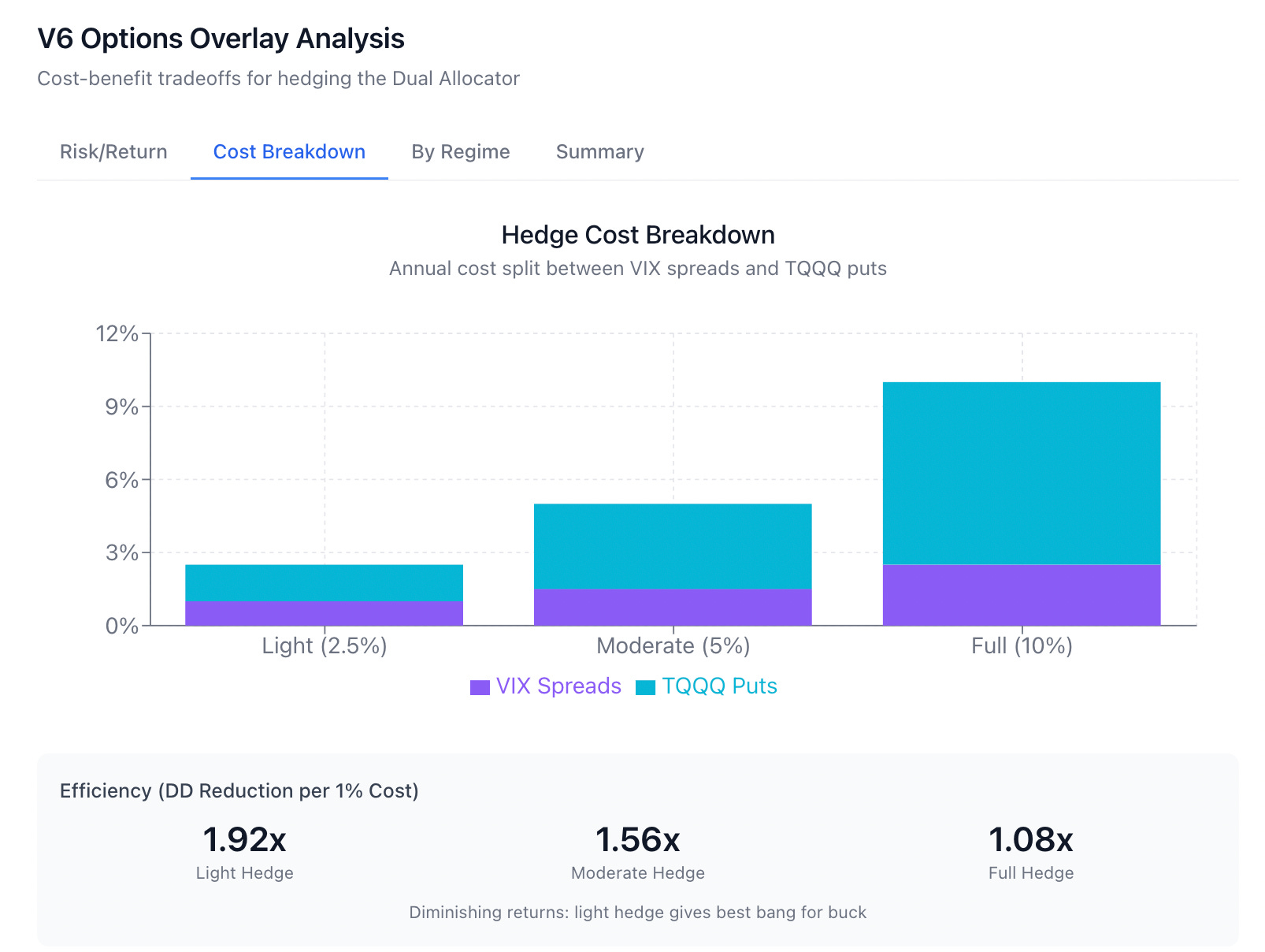
Revised Cost-Benefit Analysis
Given the math above, let’s review some more realistic projections:
Scenario 1: Light Hedge (Budget: 2.5% annually)
VIX spreads: $1,000/year (10% notional, limited coverage)
TQQQ spreads: $1,500/year (5% notional coverage)

Protection level: Modest
Max DD improvement: -5% to -10%
Projected Sharpe: 0.90 - 0.93
Scenario 2: Moderate Hedge (Budget: 5% annually)
VIX spreads: $1,500/year (15% notional)
TQQQ spreads: $3,500/year (25% notional coverage)

Protection level: Meaningful
Max DD improvement: -10% to -15%
Projected Sharpe: 0.92 - 0.96
Scenario 3: Full Hedge (Budget: 10%+ annually)
VIX spreads: $2,500/year (25% notional)
TQQQ spreads: $10,000/year (75% notional coverage)

Protection level: Comprehensive
Max DD improvement: -20% to -25%
Projected Sharpe: 0.95 - 1.00
The tradeoff is clearer now:
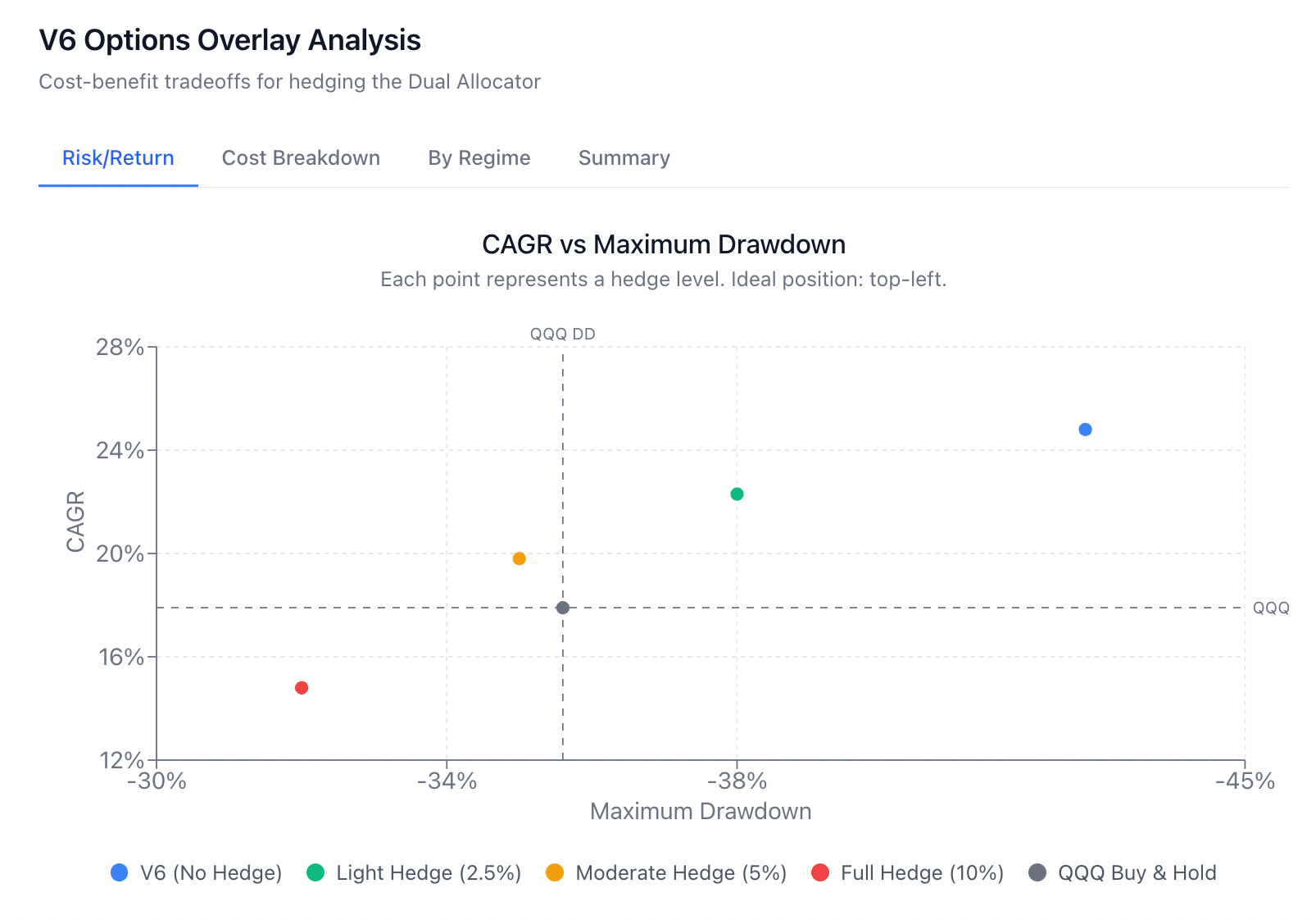
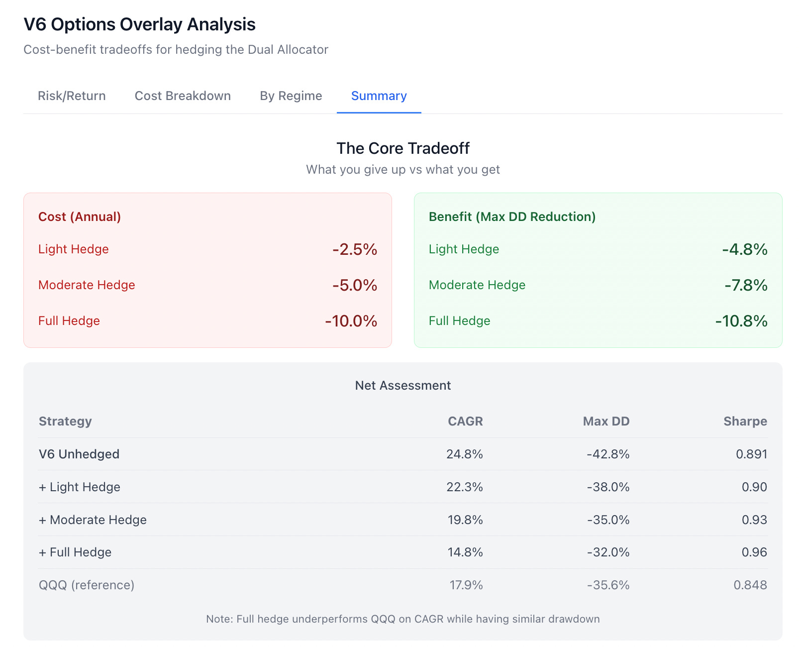
Annual Cost    Return Drag    Max DD       Sharpe (est.)
──────────────────────────────────────────────────────────
0% (base V6)   None           -42.8%       0.891
2.5%           -2.5%          -38%         0.90
5%             -5%            -35%         0.93
10%            -10%           -32%         0.96
To achieve meaningful drawdown reduction, you’re looking at 5-10% annual cost, which reduces your 24.8% CAGR to 15-20%. That’s still respectable, but it’s a different strategy than V6 alone.
When Options Make Sense
This simple cost analysis suggests options overlays are most appropriate when:
Portfolio size > $250k: Options have fixed costs (commissions, bid-ask spreads) that eat into small portfolios. At larger sizes, the percentage drag decreases.
Risk tolerance is low: If -42.8% drawdown would cause you to panic-sell, paying 5-10% annually for drawdown insurance might preserve more capital than the alternative (selling at the bottom).
V6 is the primary strategy: If V6 is a satellite position (10-20% of portfolio), I’d hedge the whole portfolio instead. Options on individual sleeves create complexity without proportional benefit.
Manage rolls: Options require active management. If you’ll forget to roll positions, you’ll either lose the hedge unexpectedly or pay extra to close early.
When to Skip Options
Portfolio size < $100k: Transaction costs and bid-ask spreads will eat 1-2% annually before you even start.
Comfortable with drawdowns: If you can genuinely tolerate -43% without selling, the 5-10% annual drag isn’t worth it. The expected terminal wealth is higher without the hedge.
My Recommendation
After working through the math, I’m less enthusiastic about options overlays than when I started.
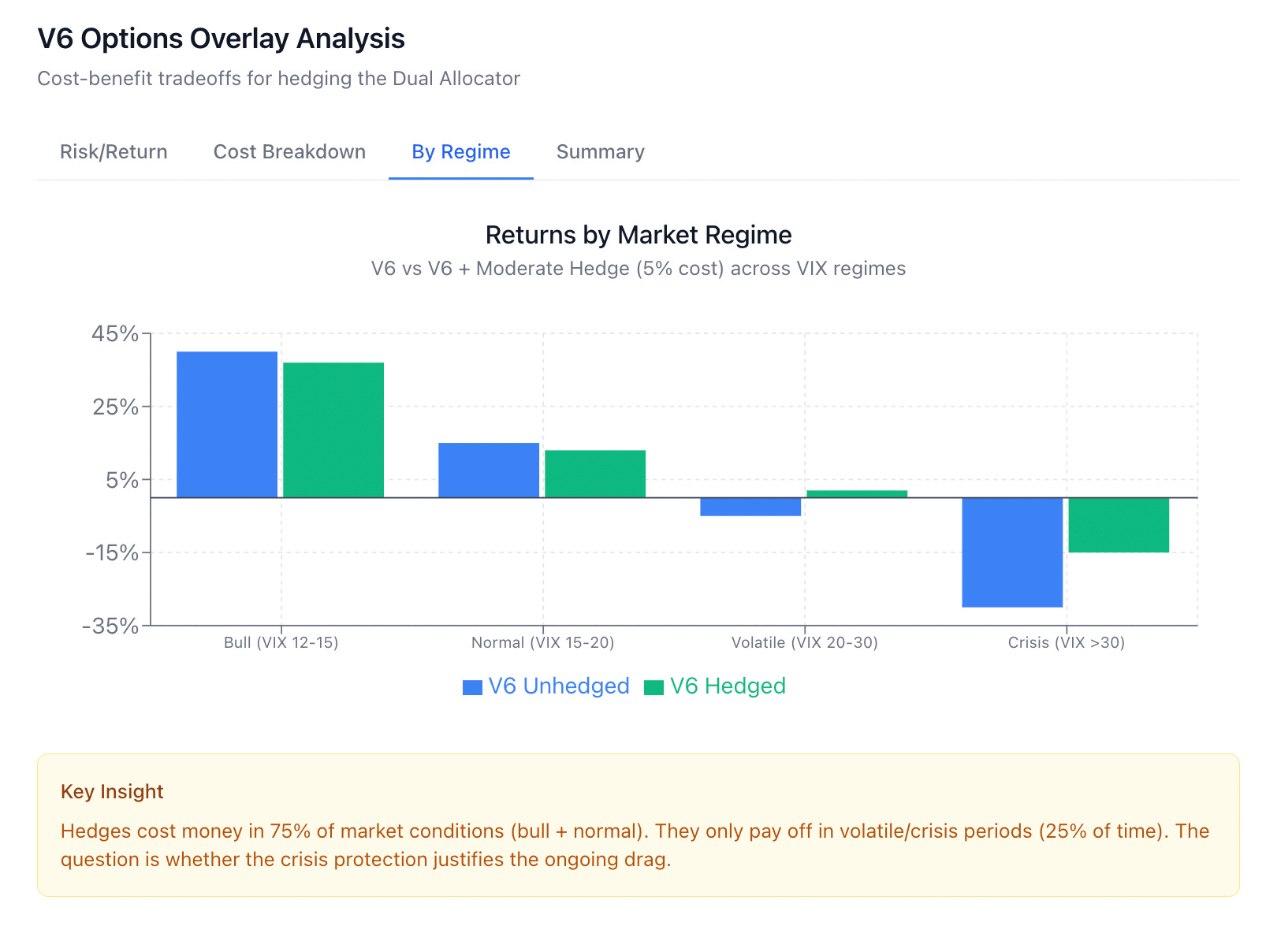
The issue isn’t that they don’t work — after all, they do reduce drawdowns. The real issue comes down to cost. Meaningful protection costs 5-10% annually, which fundamentally changes the strategy’s character.
Strategy                    CAGR      Max DD    Personality
───────────────────────────────────────────────────────────────
V6 alone                    24.8%     -42.8%    High risk, high reward
V6 + light hedge (2.5%)     22.3%     -38%      Slightly less of both
V6 + moderate hedge (5%)    19.8%     -35%      Balanced but slower
V6 + full hedge (10%)       14.8%     -32%      Conservative growth
QQQ buy-and-hold            17.9%     -35.6%    Simple baseline
The fully hedged V6 underperforms QQQ buy-and-hold on CAGR while having comparable drawdowns. At that point, you’re paying for complexity without clear benefit.
My perspective is as follows:
For most Dual Allocator V6 users: Skip the options overlay. Accept the -42.8% drawdown as the cost of 24.8% CAGR. If you can’t stomach that drawdown, reduce allocation to V6 rather than hedging it.
For large portfolios (>$500k in V6): Consider the light hedge (2.5% annually). It won’t transform the risk profile, but it provides some crisis insurance at modest cost.
For institutions or very risk-averse investors: The moderate hedge (5%) is defensible. You’re trading 5% CAGR for ~8% drawdown reduction, which is a reasonable exchange if drawdown matters more than terminal wealth.
Next Steps for Validation
This analysis relies on projected numbers. Before implementing any hedge, I’d want to:
1. Backtest with Historical Options Data
The projections assume options are priced at theoretical fair value. In practice:
VIX options have volatility risk premium (they’re expensive)
TQQQ options have wide bid-ask spreads during stress
Roll costs vary significantly by market conditions
I need historical options pricing data (CBOE for VIX, OPRA for TQQQ) to simulate actual costs.
2. Model Hedge Payoffs During V6’s Worst Periods
Specifically:
February-March 2020 (COVID crash)
September-October 2022 (Fed tightening)
Any other periods where V6 experienced >20% drawdown
Did the VIX spike precede the equity crash (hedge pays off) or occur simultaneously (less effective)? The timing matters.
3. Calculate Correlation of Hedge Payoffs with V6 Losses
A hedge is only useful if it pays when you need it. I need to verify:
Corr(VIX spread payoff, V6 daily loss) < -0.5  (ideally < -0.7)
Corr(TQQQ put payoff, V6 daily loss) < -0.5
If the correlation is weak, the hedge isn’t worth the cost.
4. Sensitivity Analysis on Strike Selection
The 25/35 VIX spread and 5%/15% TQQQ spread are starting points. I should test:
VIX spreads: 20/30, 25/35, 30/40
TQQQ spreads: 3%/10%, 5%/15%, 7%/20%
Different strikes change the cost/protection tradeoff.
5. Paper Trade for 3-6 Months
As always, real-world execution will reveal issues the backtest missed:
Actual slippage on spread entries/exits
Roll timing (is monthly optimal, or should it be weekly/quarterly?)
Psychological difficulty of paying for insurance that usually expires worthless
Summary
V6 has a 0.891 Sharpe ratio and -42.8% maximum drawdown. Options can reduce drawdowns but at significant cost.
Light hedges (2.5% annually) provide modest protection and modest Sharpe improvement—probably not worth the complexity. Full hedges (10% annually) provide meaningful protection but reduce CAGR to levels comparable with simple buy-and-hold.
The math suggests the optimal approach for most investors is either:
No hedge (accept the drawdowns as the price of higher returns), or
Reduce V6 allocation instead of hedging it
Options overlays are most appropriate for large portfolios where the complexity costs are spread over more capital and where drawdown reduction has institutional value beyond pure return optimization.
I’ll paper trade the moderate hedge (5% budget) alongside unhedged V6 for the next six months and report back on whether the theoretical protection materializes in practice.
This post is about methodology, not recommendations. Options and derivatives are complex instruments and this analysis probably contains errors. If you find them, let me know.
The information presented in Math & Markets is not investment or financial advice and should not be construed as such.