A Cross-Asset Defensive Overlay (and the Sharpe vs. Overfitting Problem)

Part 15 talks about my attempt at testing a fifth strategy of a cross-asset defensive overlay

This is part 15 of my series — Math & Markets: Building a Trading Bot.

After killing the ETF mean-reversion idea, I still wanted something that could handle choppy / sideways markets a bit better than pure trend or pure vol.

The goal wasn’t to find a magic new engine. It was to build a simple, cross-asset defensive sleeve that:

• plays nicely with my dual + vol stack,

• uses ETFs I already pull (SPY, IWM, TLT, GLD),

• stays mostly cash-buffered,

• and doesn’t require its own data center to run.

So I tried exactly that: a 20/100-style trend sleeve with a volatility gate — and then wired a Bayesian selector on top of it to choose among parameter sets.

This post is about that experiment, what the numbers look like, and a detour into Sharpe vs. ROI vs. let’s have the model do its thing without overfitting it too much.

---

1. The Idea: A Simple Cross-Asset Trend Overlay With a Vol Gate

The core concept was straightforward:

Trend-following on SPY, IWM, TLT, GLD, with a volatility gate.

Rules of thumb:

• Use fast vs slow moving averages (e.g., 10/80, 20/100) to decide long/flat per ETF.

• Only be “risk-on” when volatility isn’t screaming (via a VIX z-score gate).

• Vol-target each position (e.g., 8% annual volatility target).

• Cap any single ETF weight at 25%.

• Cap gross exposure around 50–60%, so there’s always a cash buffer.

Why bother?

• It’s orthogonal-ish to the dual + vol sleeves.

• It uses liquid ETFs I already have in the pipeline.

• It should behave better in some choppy tapes than the failed mean-reversion sleeve.

• It’s easy to backtest with the scaffolding I already built for the ETF MR experiments.

So I took the etf_mean_reversion.py harness, ripped out the MR logic, and replaced it with:

• trend signal (fast MA vs slow MA)

• optional VIX z-score gate

• same position-sizing and cap logic

• daily rebalance, minimal turnover controls

Then I started testing out combinations of various grid parameters.

---

2. The Grid: Finding a Reasonable Static Config

I ran a moderately broad grid over:

• fast MA: 10, 20

• slow MA: 80, 100, 120

• target_vol: 6–8%

• max_weight: 20–25%

• gross_cap: 0.5–0.6

• VIX z gate: 0.8, 1.0, 1.2, 5.0 (where 5.0 = basically “no gate”)

Over SPY/IWM/TLT/GLD with $10k notional, the top Sharpe cluster showed up very consistently around:

fast = 10, slow = 80, target_vol = 0.08, max_weight = 0.25, gross_cap = 0.6

Representative results from that cluster:

• Sharpe ≈ 0.85

• ROI ≈ 48–50% over the test window

• Gross exposure well-behaved, cash buffer intact

Interestingly, the VIX gate didn’t matter much in this grid — most of the best configs had very similar results whether the gate was at 0.8, 1.0, 1.2, or effectively off (5.0). In other words, with these parameters and this period, the gate wasn’t really binding.

So if all I wanted was a simple static overlay, I could stop here and say:

“Cool. Run fast=10, slow=80, target_vol=0.08, max_weight=0.25, gross_cap=0.6, ignore the VIX gate, and call it a defensive trend sleeve.”

But I wanted to see if I could be a little smarter than that.

---

3. Step Two: Add a Bayesian Selector on Top

Instead of manually hard-picking the “best” grid config forever, I tried a small Bayesian selector that could:

• look at a small universe of candidate configs,

• use simple features (VIX regime, SPY returns, volatility, trend slopes, drawdown),

• and choose which config to run per regime.

Architecture:

1. Candidate universe: ~16 configs clustered around the best grid performers (fast=10, slow near 80, with variations in target_vol, max_weight, gross_cap, VIX gate).

2. Backtest each config over the historical window.

3. For each day, label the “winner” as the config with the best next-day return (in this first pass) or best short-horizon performance.

4. Train a simple Gaussian Naive Bayes classifier using features like:

   • VIX z-score

   • 5d SPY return

   • 20d SPY vol

   • 20d and 50d SPY trend slopes

   • SPY drawdown

   • plus the VIX regime bucket (low / medium / high)

5. Regime logic:

   • Bucket days into VIX regimes (e.g., low / mid / high).

   • Only allow the selector to change configs when the regime bucket changes (to avoid wild config-churn).

6. Execution:

   • For each day, look at VIX regime → pick config predicted as best for that regime → run that config’s weights.

   • Enforce max_weight, gross_cap, vol target, and maintain cash buffer.

   • Log everything to audit + allocations CSVs.

So the selector doesn’t try to be super fancy. It’s regime-aware, not tick-aware.

---

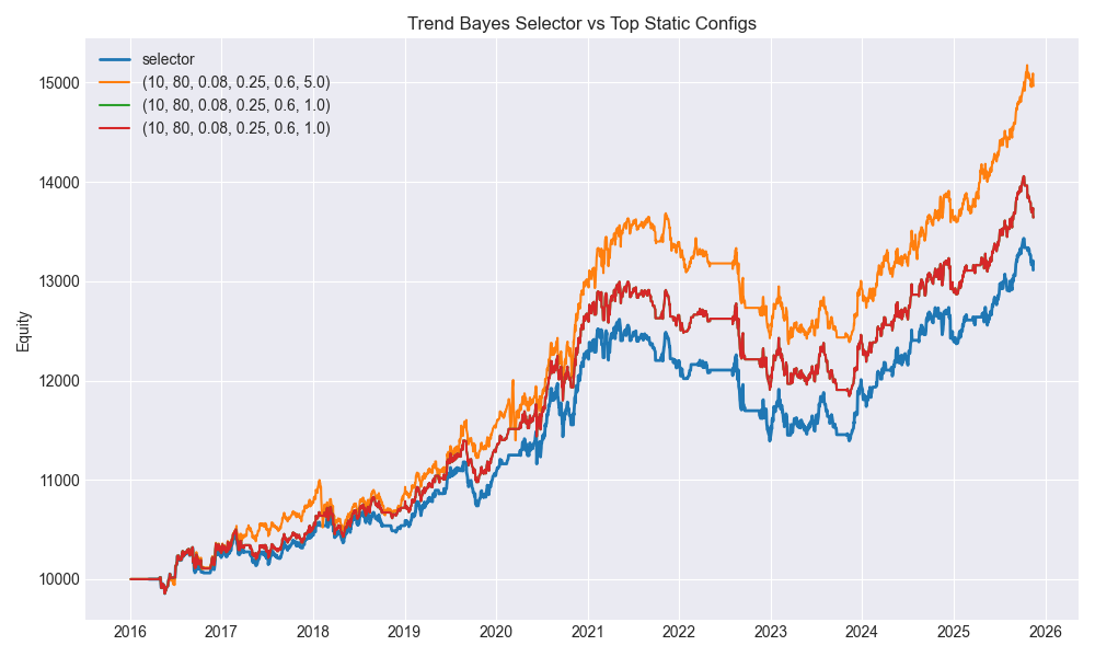
4. Results: Static Best vs. Selector Choice

From the full metrics run (2016-03-16 → 2025-11-13, 2,432 trading days), a few things stand out:

Best static config in the grid

• Config: (fast=10, slow=80, target_vol=0.08, max_weight=0.25, gross_cap=0.6, vix_z=5.0)

  • Here, vix_z=5.0 basically means “VIX gate off.”

• Sharpe: ≈ 0.883

• ROI: ≈ 49.66%

This is the top Sharpe static config over the full sample.

Selector’s chosen config in the latest run

The selector, however, didn’t just hard-lock onto that one. For the final regime (classified as “high” VIX), it leaned toward:

• Config: (fast=10, slow=80, target_vol=0.08, max_weight=0.25, gross_cap=0.6, vix_z=0.8)

• Sharpe: ≈ 0.66

• ROI: ≈ 31.13%

• Final total: ~$13,112 on $10k (after introducing forward-validation + richer features)

Meanwhile, the selector logic:

• trained on next-day returns / regime behavior,

• only switches when VIX regime changes,

• and doesn’t optimize for “best full-history Sharpe.”

So the “best full-period Sharpe” config (vix_z=5.0) isn’t guaranteed to be the one the Bayesian selector settles on for the current high-vol regime. It’s choosing what it thinks is best conditional on current conditions, not best in hindsight.

---

5. Why Not Just Force the Best Sharpe or Best ROI?

At this point I had a conversation with a quant friend (who has way more degrees than any one person should reasonably have), and we got into the classic problem:

What exactly are you optimizing for? And how much do you trust your backtest?

Sharpe looks good enough on paper. ROI looks good enough in a chart.

But the moment you hard-code “always pick the best Sharpe” or “always pick the best ROI” from the same backtest you used to define the universe, you’re halfway into overfitting territory.

A few issues:

• You’re implicitly rewarding noise that happened to look good in-sample.

• You’re training on the same data you’re choosing from (confirmation bias).

• You’re conditioning your whole system on a single, cherry-picked path of history.

The selector I built is intentionally dumb in a very specific way:

• It uses simple features.

• It labels based on next-day behavior, not full-history Sharpe.

• It only switches on regime changes, not every tick.

• It now includes a forward-validation split (train on earlier chunk, validate on a later chunk).

It’s not optimal and it’s not max Sharpe. But it’s good enough to not be obviously overfit given the limited data and simple features.

I could possibly bias it so that, within each regime, it tilts toward the best full-history Sharpe among configs in that regime. But my friend pointed out that you will end up creating models that work well in the context of the data they were trained on vs. net new data.

---

6. Where I Want to Take This Next (Synthetic Data and Testing Discipline)

The real answer to the Sharpe-vs-ROI-vs-overfitting question is: you don’t really know how robust your model is until it sees data it wasn’t born from.

Right now, everything is still being tested on the same historical tape:

• dual sleeve

• vol sleeve

• Bayesian blender

• ETF trend overlay

• and now this Bayesian trend selector

As a next step, I want to get more serious about how I test models, not just which models I test.

Specifically:

1. Generate synthetic data.

   • Not cartoon-random series, but statistically similar paths (e.g., simulated returns with similar vol, autocorrelation, cross-asset correlations, and regime shifts).

   • Enough variety that the model can’t just memorize one tape.

2. Train on one sample, test on another.

   • Build the selector (and future models) on one “world.”

   • Evaluate it on a completely different “world.”

   • This is the only way to see if the model is learning behavior, not just memorizing noise.

3. Try different evaluation lenses.

   • Sharpe is good, but not everything.

   • Look at drawdown, turnover, regime-specific performance, and “how often the model is roughly right” in picking the better config.

   • Explore rolling-window Sharpe as a label instead of raw next-day returns.

Only then can I have more confidence that “best Sharpe in backtest” means something useful out-of-sample — and that a Bayesian regime selector isn’t just overfitting a handful of parameters to one historical decade.

---

Closing

The cross-asset defensive overlay experiment was a good reminder of why this project exists in the first place:

• The simple 10/80 ETF trend sleeve with vol-targeting and caps actually looks decent.

• The VIX gate didn’t matter much in this window, but the structure is sound.

• The Bayesian selector adds a bit of regime-awareness without trying to be too clever.

• The static best Sharpe config exists — but hardcoding it feels like a trap.

So for now, I’m keeping:

• the 10/80 trend overlay in the toolbox as a candidate defensive/orthogonal sleeve,

• the Bayesian selector as a reasonable way to choose configs without going full curve-fit,

• and, importantly, a growing suspicion of any model that looks too clean on a single backtest

The next step is not “squeeze more Sharpe out of this with one more tweak” but rather to build better ways to test models so that whatever survives has a chance of working when the market stops looking like the last ten years.

Synthetic data, out-of-sample regimes, and more deliberate validation are up next.

One model at a time.

The information presented in Math & Markets is not financial advice and should not be construed as such.

---